asymptotichigh5

[asymptotichigh5]

Energy, the economy, and everything else.

I’ve been meaning to address this subject somewhere for a while. For the longest time, I hesitated on what the best medium to achieve this would be : on one hand, a Facebook status needs to be short and concise, which is not necessarily my forte and of course, there is also the fact that it would quickly be washed away in the storm of social media posts that has become 2020. A YouTube video then occurred to me to be most appropriate, but it would be long, my camera sucks and I hate video editing. So, I finally turned to this blog, which I had abandoned for quite some time. Surprisingly, there was an article in my drafts I had started writing almost 5 years ago about exactly this topic titled “A physics crash-course for politicians: a recipe not to kill us all”, but it was a bit too dramatic and I might get called off for taking political stances, when in reality there will be none in this post (which is surprising, for any of those reading this who know me). Anyway, this article will be the first in a series, which I might or might not continue, depending on interest, even though I did promise a friend of mine to carry through the entire message the whole way through, hopefully I’ll be able to do this with some of you actually reading all the way through, though that might be too optimistic.

Energy is a concept which is as important (if not more) as it is misunderstood by the general public. Most people don’t consider energy to be a considerable issue in their daily lives, but hopefully by the end of this post you will understand that energy is what allows you to live your 21st century carefree lifestyle. It turns out that most of us consider energy to be a bill to pay at the end of the month, or an annoyance to pay for when we fill our cars with gasoline at the pump, but energy — before being a bill to pay, or a commodity — is a physical quantity. A quick look at Wikipedia will give you a definition of energy which appears to be rather circular. Perhaps a more appropriate definition of energy for the sake of this post is the following:

Energy [/ˈɛnədʒi/, noun] : a physical quantity quantifying the ability to change the environment, or the ability to do work.

By “change the environment” we refer to the ability to perform any kind of change at all. Letting a ball fall involves energy, heating up water to make a cup of tea involves energy, me typing on this keyboard at this very moment also involves energy, etc. The SI unit for energy is the Joule, which at the human scale represents a tiny bit of energy (roughly speaking, it is the energy required to lift a medium-sized tomato (300 grams) by 1 metre. This unit has the annoying nuisance of being too small, so for the rest of this post we will talk about energy in terms of MWh (megawatt-hours), which corresponds to 3 600 000 000 Joules, which is a hell of a lot more medium-sized tomatoes lifted, or in terms of kWh (kilowatt-hours), which corresponds to 3 600 000 Joules. It is a good exercise to try to understand the MWh in terms of human work to put everything into perspective. To this effect, the BBC actually had a great documentary which appeared in 2009 about electrical energy consumption in the UK which performed an experiment in which a tiny army of people were forced to pedal to provide electricity to an average-sized house with an average-sized family having an average-sized consumption of electricity. While the documentary has great shock value, we need not hire an army of 80 cyclist to get the right orders of magnitude. An 80 kg man carrying 10 kg of supplies with him and climbing 2000 m up a mountain spends roughly 0.5 kWh to go up the mountain. Similarly, digging up 6 m${}^3$ of dirt to make a hole 1 m deep takes roughly 0,05 kWh of energy. By comparison, 1L of oil provides 2~4 kWh of (usable) mechanical energy.

Of course, using the oil to drive up the mountain, or to fuel an excavator to dig up the holes is a no brainer. Oil, or more precisely the machines it feeds, are not constrained by fatigue, do not form unions, do not complain that the ruble is too heavy, or that their legs are tired. It is also incredibly cheap by comparison, even if the human workers going up the mountain or digging up the hole are not getting paid at all. Assuming the cost of a slave to simply be the sustainance cost of a human being (i.e. minimal clothing, food and shelter) it is still a couple of hundred times cheaper to use a machine instead of a person to perform tasks, whenever possible. The reason why slavery ended is not because all of a sudden people grew a conscience out of thin air, or because we are so much better or educated than our ancestors ; it is simply stupid to have slaves in a world where you have access to a dense source of energy, because using this energy for mechanical work is many times more efficient and cheaper than owning slaves. This heuristic argument is also what ultimately explains the correlation between the abolition of slavery and the first industrial revolution (although the latter was mostly fed by coal as opposed to oil). In other words, the huge disparity in the efficiency of dense energy sources is what explains that mankind has historically always transitioned to sources of energy which monotonically increase in energy density.

But just what makes energy so important? Well, the answer lies in the definition. Since energy is ultimately the driver for any transformation of the environment, energy is by definition the main driver of the economy, too. In fact, the availability of a large supply of energy is what has allowed the development of modern society as we know it: paid holidays, retirement benefits, social security, social programs, your trip to Thailand last year, the variety of food you find at the supermarket, the fact that you even have disposable income to spend however you wish, free time, your ability to pursue long years of study, etc. Without the access to a cheap, reliable source of energy, this would all be impossible. Without realizing it, on average, we can calculate an equivalent amount of slaves used by any human on Earth today, given our estimates on the output of energy a human being is capable of delivering above and the total energy consumption of the planet. Doing the math, we find that an average human lives as if he/she had ~200 slaves working for him/her constantly. If we look at developed nations, this number jumps to 600 to 1500 equivalent slaves. This is an outstanding standard of living compared to what any of our ancestors ever knew. And so, it’s not that our generation is 200 times more productive than previous generations of humans, what has been driving the economy for the past 220 years is not humans, so much as it is the increasing access to a park of machines which has driven GDP growth since the industrial revolution. In fact, this can also be seen in developing countries, where an increase in development is immediately accompanied by a rural exodus driven by the introduction of machines to perform the heavy work in the fields. This allows for a widening of the pool of workers, which can then be free to use more machines and increase GDP.

So what sources of energy have we been exploiting in the last 220 years? Worldwide, the mix looks a little bit like this: 

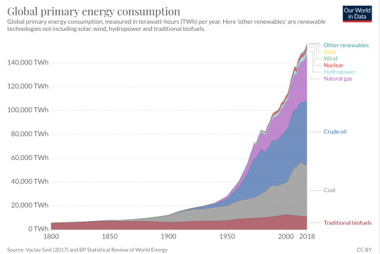
Notice that most of this mix (oil, gas and coal) are sources which are fossil fuels. In essence, what this chart is saying is that we owe all of the societal progress of the past 220 years to fossil fuels. Of course, the use of these fuels has the annoying consequence of releasing CO${}_2$ into the atmosphere which — as we know — has some rather undesirable consequences for the future of humanity. This chart also tells a story about how people have completely misrepresented and misunderstood the problem. Most people think that the energy crisis will ultimately be solved by replacing the carbonated sources of energy by “renewables”, even though the later are basically invisible in the above chart. Luckily, a world where we live only with renewable energy is entirely possible: it’s called the Middle Ages. The impossibility of replacing these carbonated sources with “renewables” is an important point to treat, and deserves an article of its own, but in the end its cause is the same as what has driven this discussion so far: energy density. We shall come back to this important point in a subsequent post. For now, let us finish driving the point home in establishing the unequivocal link between energy, specifically oil, and GDP.  Energy availability is the main driver of the economy, this is simply because the economy is nothing other but the collective transformation of stuff into other stuff by humans. This, and the fact that 50% of the world-wide oil consumption is used to transport goods or people from point A to B is what explains the following correlation between oil and GDP: 

In light of global warming, the question becomes one in which we are forced to arbitrate between real GDP growth and carbon emissions. It is literally that simple, yet it is difficult to grasp what this means. GDP growth is an abstract concept most of us don’t really understand, and most people advocating for giving up growth don’t fully grasp the consequences of what it will mean for all of us. Very really, what it means is diminishing real wages and purchasing power by a factor varying between 3 or 10 over the next 30 years (we will come back to these figures eventually in another article, too). Now, most people will point out that we can and should just take all this wealth from the oligarchs and the billionaires out there, and this is true and should definitely be done, but it will unfortunately still not be anywhere near enough to solve the problem. Orders of magnitude are a bitch and maths sucks, especially when they contradict your political opinions. In real terms, giving up growth means to take your current salary, and divide it by 10, and ask yourself whether you are really ready to live with that. The questions on left and right are at this point so irrelevant that it is stupid to even ask them. Both of these models of thinking completely rely on a pie which is ever increasing and in which the living standards of everyone eventually rise. For the right, this is obvious, but this holds true even in a leftist society, in which the social programs and everything that goes with it relies heavily on economic growth and an increase of the economic pie. This view is flawed, as in very real terms in order to protect ourselves from climate change, the only way is to considerably decrease our dependence on fossil fuels, in other words, considerably decrease global GDP.

(Un)fortunately, whether the politicians decide to take global warming seriously or not, the problem will auto-regulate eventually. You see, there is a tiny and obnoxious problem regarding our addiction to fossil fuels: we are running out of them. We should point out that not all fossil fuels are equal: this is not only true from a carbon emission perspective, but also from a transportation point of view. Indeed, only about 10% of the coal produced yearly is actually exported, because it is inconvenient to transport. Gas presents a similar problem, given its physical form, which is not sufficiently energetically dense to be easily shipped without compression (which itself involves energy). This leaves oil as the main source of energy which is actually exportable and tradable.  And so, not only is oil vital due to the fact that it is the only source of energy which can reliably be used to for transportation, it is also the only option when looking at trading energy internationally. However, oil production has been already past its peak in most countries with considerable oil reserves. From a European point of view, the problem is actually worse as the energy consumption in Europe has been stagnating and in fact decreasing since 2005, when we reached peak consumption.

Incidentally, this explains why there has been no -- and there will be no -- economic long term real growth in Europe in the future, and it this has indeed been the case ever since 2008. In fact, most of the economic growth which has happened in Europe ever since is due to the trade of goods which increase in value over time (such as housing), which gets further gets inflated as there is a surplus of liquidity which has been continuously injected into the system since the introduction of quantitative easing. We will come to this problematic in a latte post. Similarly, we observe analogous curves of decrease in variation of energy consumption in the countries of the OECD (source of data: BP Statistical Review 2017), which means that this halting of real economic growth is not to be expected anywhere else in the OECD either.

During a recent discussion with a close friend of mine, he pointed out that the decrease in consumption in energy could be explained by the fact that the economy in developed countries had essentially become an economy of services, and that thus, this correlation between GDP and energy consumption and production was flawed, but this reasoning is wrong. First, because many of these services introduced involve or depend strongly on developments in e-commerce and industries attached to the development of the Internet and computers. However, the digitalization of the economy has not led to a decrease in energy demand, but in fact quite the opposite, if anything it has considerably increased our energy dependence. Second, the data simply states otherwise across the board. For instance, the chart below depicts an evolution of the percentage of people working in services and the amount of tons of CO${}_2$ released in the environment per capita in the World (data is from the World Bank).

Of course, the fact that these are positively correlated in the world and these countries is expected. In the world, because supporting the increasing living standards of the people working in the service sector necessarily comes out of an increase of the economic pie, which can only mean that the energy consumption (thus, at first order, the tons of CO${}_2$ in the atmosphere) increased. In European countries, the CO${}_2$ per capita has been reduced, partly to a negligible population growth, but also due to the delocalization of the most polluting elements of the economy to developing countries. Nonetheless, the general worldwide trend is clear: more service sector employment correlates with higher output of CO${}_2$, which implies higher energy consumption. But of course, by the reasoning above, this is hardly surprising.

Most of the time, the decline in the rate of growth of oil production is dismissed by saying that we will always find alternative forms of petroleum which will remain exploitable and will secure us with more oil. However, these alternative sources, such as bituminous sands and are problematic to exploit, require more energy input to be exploitable and are of lesser energetic quality. Similar decreasing curves of consumption and production have been appreciated for gas as well. Coal remains an exception to this, but it is not easily tradable, which implies that only 8 countries (including the US, China and Australia) really can consider exploiting coal for long term energy consumption, but given the climate consequences this poses, this is hardly a desirable outcome.

And so ultimately, it is not even a question of deciding whether or not we want to transition out of fossil fuels or not. The decrease in fossil fuel consumption will happen whether we like it or not — and by extension, so will the inevitable shrinking of the economy. The problem is that it might not happen fast enough to avoid catastrophe, which might already be unavoidable. What this also means is that the questions we should be asking ourselves as a society are not so much whether we should adopt liberal or leftist policies, but rather how we optimize the distribution of resources in a world where the economic pie decreases year by year, but no one seems to be wanting to have this discussion seriously.

#energy #energy crisis #renewables #renewable power #oil #environment #environmetalists #economy #economic crisis

[asymptotichigh5]

Hope…

“Here’s what the Electoral College map would look like if only millennials voted”

[asymptotichigh5]

Don't forget to go out and #VoteRemain today! #UK #London #StrongerIn #Remain #europe #EU #strongerineurope #parliament #bigben #afternoon #tbt #throwbackthursday #throwback (at Big Ben)

#europe #voteremain #parliament #throwbackthursday #strongerin #tbt #strongerineurope #throwback #remain #london #afternoon #uk #eu #bigben

[asymptotichigh5]

Yesterday, while taking public transport, I asked myself why it was that we always have the impression that we have to wait the longest time possible for a bus or a metro. After thinking about it for a while, I realised that the arrivals of public transport can be modelled as a Poisson process. It is really no surprise that the expected value of the time to wait to would simply always be the average time between buses/metros. Hence, it really was no surprise that we must always wait the "longest" time for a bus. #poisson #montreal #metro #sherbrooke #quebec #station #prochainestation #bleu #metrodemontreal #probability #statistics #math #appliedmath #buses #publictransport (at Sherbrooke (Montreal Metro))

#bleu #metrodemontreal #sherbrooke #probability #metro #buses #appliedmath #prochainestation #station #quebec #poisson #statistics #publictransport #montreal #math

[asymptotichigh5]

Dogma vs Bayesianism: the modern battle between religion and rationality

I know this post will be quite controversial and diametrically opposed to what this blog was originally supposed to stand for. I never meant for it to go political in the first place, but in view of the recent events that have occurred and in particular their frequency, I think it’s time we addressed a couple of problems.

First off, I just wish to say the following: these is just my personal input on the topic. If you happen to be a fervent believe in any type of religion, I respect that, as long as you don’t impose it to anyone else, hopefully you’re just able to appreciate this read with a critical eye.

Here is why I think we should get rid of religion all together. Now by religion, I am not targeting a single group, not the Muslims, not the Christians, not the Jews, no. What I am targeting here is not people; I am targeting an idea: institutionalized, dogmatic religion (i.e. a non-bayesian belief system).

Now mind you, the distinction is important. As you will see later on in this post, there is a distinction between believing in God and adhering to institutionalized religion. This article is about criticizing the later, not the former. I think for too long we haven’t dared to question these institutions enough and I think it’s time we sat down and had a rational discussion about it.

The inconsistency of religion as described by Holy Books

The first point I wish to address is the irrationality of adhering to any particular religion. 

In its purest forms, religion is a dogma. It is something you should accept and incorporate in your belief system without question and, in principle, no amount of evidence should waver your belief system. Now, some of you might argue and say that in practice, religion is something that can be interpreted in a variety of different ways and so it poses no harm at all. And you’re right, it is open to interpretation. On the other hand, it is so open to interpretation that most individuals allow themselves to essentially cherry pick what parts of the scripture to believe or not, to the extent that the entire system becomes not only superfluous but also inconsistent.

The best example of this is that many priests and religious leaders believe in miracles written in the bible as if they were fact. On the other hand, when confronted to the moral code that is written on the same book as the “word of God”, they are willing to give themselves the freedom of choice. But logically, that doesn’t make any sense at all! 

How is it logical to adhere to only parts of a book that is supposed to be the “absolute truth” and that was written by a perfect being that makes no mistakes at all? The fact that an omniscient, all-knowing being would be so vague in his own scriptures as to leave room for interpretation in the first place shows flaws in this “perfect” being. 

Worse, who are these humans to allow themselves to bend the words of this hypothetical all-knowing being’s instructions on how to live life and why is it that they have authority to do so above any other individual?

If God did in fact exist, or let alone write any of these books, wouldn’t have he ensured himself to give clear instructions that leave little room for the imagination? Once again, we reach a contradiction in this belief system and this time from a completely different direction. The conclusion in both cases is the same: simply stated, by opening the Bible, the Quran and other holy books to interpretation, one is admitting that God is imperfect, as he could haven not possibly foreseen what was to come. However, this breaks the hypothesis of the existence of this hypothetical creation being perfect all knowing, since we have just shown he was flawed in his scriptures to begin with. 

This is of course, not even starting to touch all of the inconsistencies and logical fallacies that one can find in, say, the bible itself when one examines it closely.

The existence of God and its irrelevance

Next I wish to address the belief in God. About this I can only say: believe whatever you want. This question is undecidable, in fact, there is no point of even having an opinion on this topic and therefore the concept of God itself becomes completely irrelevant to begin with. To illustrate why I think it’s simpler to begin with a thought experiment. Suppose I told you that there is a purple dragon in the room you’re currently in. You would then proceed to ask, well, if that is the case, then why can’t I see this dragon? To which I will reply that he is invisible. But then you object and you wish to know why you cannot hear him. To which I reply that the dragon never makes any noise at all. You argue, still, in frustration: “why doesn’t he dissipate any heat?”. To which I reply that he doesn’t, in fact, dissipate any heat at all! He’s perfectly insulated. We continue arguing ad infinitum in which you ask me why you cannot perceive this creature or why this creature has no influence on its surroundings, to which I can come up with an infinite amount of excuses. After an infinite number of steps in such an argument you realize that the existence of this dragon is actually irrelevant to your own existence, as there is no way you can ever interact, perceive or do anything with this dragon. In addition this dragon has also no impact on anything that could ever possibly affect your existence, therefore whether the dragon exists or not is simply a matter of choice. You can believe he exists, but this will not – and should not – influence any further logical perception you can make, or by contrast you can choose to believe that he doesn’t exist, but once again it makes no difference whatsoever to your existence thereafter. For convenience though, it is easier to choose not to believe in such creatures, as I can come up with an infinite amount of different creatures with the exact same properties and call them different things, but this is just clutter in the language of your logical system that is irrelevant, as whatever you can proof in these different models of reality is exactly the same (model and language in these case are actually mathematical terms taken from Model Theory, which I encourage you to investigate).

You see, some questions are stupid questions. Questions that will never have an answer because they are undecidable. Personally, I am quite bayesian in my beliefs on the existence of God, and insofar as I’m concerned, he is exactly like the dragon, until I can see evidence of his existence. Then, I’d be more than happy to change my belief system accordingly. (Un)fortunately though, no such evidence exists.

However, there is a clear distinction between this belief in God, which is purely an addition to the language of the logical system used by an individual and the addition of dogmatic religion, which affects the believe system at its core by installing a permanent version of what an individual perceives as true. This contrasts the ideal model of a rational, empirical person, which would take into account all new evidence and would switch its belief system in accordance. 

Why is this system better than the dogmatic one? Because at the base, we have no way of knowing what the absolute truth of things is. The best we can hope to do is to think something is right after consistently observing things are a certain way. This is how cognitive beings actually learn. 

A simple illustration on how these two contrast each other: you drop a ball and wait for an outcome, now, you notice that it falls. Then you do this multiple times and notice that the ball always seems to fall. Moreover, this event is independent of the object at hand. Therefore, you have elaborated a probabilistic outcome in which things fall when you let them go. Each time you observe this happening again, it reinforces your belief in the fact that things fall when they fall, therefore, such a cognitive being would not deem it wise to jump off a building, so that he doesn’t fall to his death and subsequently die. 

On the other hand, let us pose the hypothesis that another individual adhering to a dogma which states that things never fall to the ground. This individual can then do the same experiments as the bayesian individual, on the other hand, he will always reject the outcome of the experiment and keep his belief system intact. If you then asked this individual to jump off a building, he will do so with confidence, as he still believes that he will not fall and subsequently die in the process.

Now this might seem like a silly example: but it is no different than the people who deny themselves clinical treatment for religious reasons, or people that refuse to believe in evolution given all the evidence that exists to support this theory or people that refuse to vaccinate their children and the list goes on and on… Terrorists are nothing but individuals who have adhered to an extreme dogma and refuse to intake any evidence to switch their beliefs away from what they think. 

Religion as a social anchor for morality

Some might argue that religion provides a moral anchor to society and that without it, many individuals would be left without some kind of a moral compass. About this I only have to say that you don’t have to fear the existence of a place of eternal damnation to adhere to a particular moral code. If this was the case, atheists would be immoral beasts. But giving that as an explanation is way too simplistic. We must ask ourselves from where does morality actually arise.

The first thing to say is that we can ground morality in biology. Indeed, evolutionarily speaking, morality and altruistic behaviour poses a challenge to be explained. However, there are studies by biologists which show that we can ground morality in evolutionary biology. Indeed, altruistic behaviour favours the survival of species, which is why we can observe moral codes in not only our species but also in animals as well. However animals, contrarily to us, don’t have dogmatic religion as a moral compass, but they can still distinguish “right” from “wrong” (the definition of these of course, varies extensively). 

That is to say, morality doesn’t depend on religion at all. It is not fear of God that prevents people from killing each other off… Thinking so would be naïve given the amount of wars and murders that have been committed in the name thereof (which by the way poses another contradiction.. God says not to kill but somehow it’s okay to kill if you’re killing for him?)

The sole fact that society’s moral code has been changing vastly over the centuries is proof that there is no definitive moral compass that we should keep intact. Morality, much like everything else, is also very much Bayesian. It changes with the income of new evidence. 

And yes, to some extent religion has played a part in dictating society’s moral compass, but what I wish to stress is that it is in no way a necessary means to do the latter. In particular now, where morality has been forced to change incredibly quickly as new technologies and concepts emerge. While the world’s major religions have made some efforts to change their moral compass (which again, is contradictory to what these institutions even stand for) they are incredibly slow and inapt at doing so. They have become a cumbersome obstacle for new moral codes to emerge and often times only slow down social progress. 

Religion is not necessary, but…

Religion, as we I have argued, is thus not necessary for society to function. On the other hand I wish to stress a couple of things. 

First off, belief in God is not what I mean by “religion” in this post. Although it has been shown that belief in God statistically decreases with education, it is not eradicated. That is, it could be that belief in a superior power is inherent to some individuals who have some kind of predisposition to this. If this is the case, then so be it. Like I stipulated earlier, it is not the belief in God that I am criticizing, as this is not what affects the rational capacities of an individual, but rather everything that religion seems to impose with that particular belief.

Further studies into the biological reasons of the existence of religion should be pursued and investigated, as well as what was mentioned above, the fact that the belief in God doesn’t disappear and seems to be inherent to some individuals (this however is not known, it is just a hypothesis of mine). 

Finally, the main reason why it would be great if the world had no religion is because then humans could finally perceive to be more like each other, as they are instead of creating barriers between themselves. However, it would be naïve to think that all barriers and that discrimination would disappear if religion didn’t exist, but at least it would be one less thing to worry about. In any case, we should all work towards being more tolerant towards each other and be ready to have discussions about all beliefs, including religious ones.

#religion #bayes #bayes theorem #bayesian statistics #islam #christianism #christianity #religious #hinduism #buddhism #sects #radical islam #radicalisation #radicalization #radical christianity #radical #dogma #dogmatic #atheism #agnostic #agnostism #opinion

[asymptotichigh5]

Rainbows happen whenever light refracts and then internally reflects within droplets in the air. The angle between the source of the light and the observer is always approximately 42°. I guess some of the most beautiful things are just not naturally straight. #orlandoshootings #orlando #support #pride #rainbows #walks #coffee #afternoons #science #burn #gayinsta #skyline #sunset #damndaniel #cloud #sky #weather (at Brossard, Quebec)

#coffee #rainbows #support #burn #orlando #afternoons #orlandoshootings #skyline #weather #sunset #cloud #sky #walks #pride #gayinsta #damndaniel #science

[asymptotichigh5]

So I was out today and I saw a beautiful yellow moon. I then pondered why it would be that the moon would appear yellow on some particular nights and not in others. Quickly I realised that this was simply because of the moon's position close to the horizon: the answer was thus simple, Rayleigh scattering. Basically, the scattering cross-section (which in some way quantifies the amount of scattering and which we can derive from first principles using electrodynamics) depends on the inverse 4th power of wavelength. This means blue light (shorter wavelength) gets scattered much more than red light. This is why when we look at the moon close to the horizon, it appears to be redder (i.e. yellow) than usual. Some might argue that physics takes away from the beauty of nature, but in my opinion understanding nature only contributes further to its beauty.

[asymptotichigh5]

[asymptotichigh5]

On dealing with large degrees of (procrastination) freedom (Part V)

Read Part I here

Yay! Part V of this series. Who would’ve thought that it would’ve gone this far. Before I get into describing statistics I must talk about something that just crossed my mind. For no particular reason other than the fact that it’s tumblr. You know what’s really annoying? When people write IIII in roman numerals instead of writing IV. Like, didn’t you go to primary school to learn that 4 in roman numerals is IV? And they make clocks like this? What is wrong with the world?

Anyway, without further ado, let us start by considering the next step in our journey to provide rigorous framework for thermodynamics. But first, I feel like I left off a very important thing on the last post and I wish to make amends for it so we shall talk about spheres instead. Now you might think “Daniel, this has nothing to do with Thermodynamics” (yes, my name is Daniel, for the unknown readers). But it does. And it’s fun because we’re not going to be talking about any old boring 3-dimensional sphere. We’re going to talk about the n-dimensional sphere! There are many things that we could talk about, but I wish to focus on the hypersurface of the sphere. In particular what were are concerned with is the solid angle of the hypersphere. 

To do this, we will consider Gaussian integrals. I will denote the solid angle of the n-sphere by $S_n$. Let us suppose we wish to integrate over all of $\mathbb{R}^n$:$$ I_n = \int \prod_{i=1}^n dx_i \exp\left(- \sum_{i=1}^n x_i^2\right) $$We can notice that there is a symmetry in this integral by virtue of the fact that the gaussians provide natural rotational symmetry. Thus, this motivates the simple change of variables: $r^2 = \sum_{i=0}^n x_i^2$ (here, as you may have guessed, $r$ denotes the radius of our n-sphere. Now the differential volume element $dV_n = \prod_{i=1}^n dx_i = S_n r^{n-1} dr$. So then we have the following result by also noticing that all the contributions from each of the $\int dx_i$’s are the same, and they are all independent from one another so that we may split the integral:$$ \int_0^\infty dr \, e^{-r^2} S_n r^{n-1} = \left( \int_{-\infty}^\infty dx \, e^{-x^2} \right)^n $$On one hand, we know what the result of the Gaussian integral is over $\mathbb{R}$ is, and we note that $S_n$ is just a numerical factor that does not depend on radius so we may take it out of the integral. Additionally, we note that on the left hand side, we actually have $\frac{1}{2}S_n \Gamma(\frac{1}{2}n)$, because $\Gamma(m) = 2 \int_0^\infty dr\, e^{-r^2} r^{2m-1}$. This means that overall (evaluating the Gaussian integral on the right) we have:$$S_n = \frac{2 \pi^{n/2}}{\Gamma(\frac{1}{2}n)} $$

Great! So now we have found the solid angle for the n-dimensional sphere, but what exactly have we gained? Well, if you recall, last time I was arguing that $\Omega$ actually corresponds to the hyperarea of the surface in phase space corresponding to the constraining condition $\mathcal{H}(\mu) = E$. I then claimed we could take a small $\Delta E$ around it and actually look at that shell instead and that the error would be negligible. Here, I wish to further motivate why in concrete terms (ok not going to lie also felt like deriving stuff for the n-dimensional sphere because I won’t be tested on it but I find the idea really cool). I suppose this is best illustrated by an example. Suppose we had the ideal gas (oh, you thought I wasn’t going to talk about it didn’t you!). In any case, for this relatively simple system, we have that the Hamiltonian is simply dependent on the momentum of the particles: $\mathcal{H} = \sum \frac{p_i^2}{2m}$. We can thus see that over the integration over phase space, we’ll only have an integral which will be essentially over a hypersphere with radius $\sqrt{2mE}$ in $3N$-dimensional space ($N$ is the number of particles in the system). There will be another contribution from the integral over the coordinate space, which will yield a factor of $V^N$. If we compute the integral (which is a bit tedious) we have the following result ($K$ will denote that the integration is over the restrained space):$$\Omega(N,V, E) = \int_{K} \prod_{i=1}^{3N} dq_i dp_i = V^N \frac{2 \pi^{3N/2}}{\Gamma(3N/2)}(2mE)^{(3N-1)/2}\Delta E$$We however are interested in the entropy, as we discussed in the last section, so as you can see when we do this, we obtain simply that the entropy will only acquire a factor of only $\ln(\Delta E)$, which is at worst (if you let $∆E$ be basically the entire radius of the hypersphere) $\ln(\sqrt{2mE})$, which is negligible compared to all the other terms which scale with $N$. This is great... But it’s wrong.

You see, as it is, we have a problem with the additivity of entropy. I won’t go through the details but roughly speaking, the problem happens when we mix two gases that are identical and have the same density. Then in that case, the above expression predicts that there should be an increase in entropy. But this doesn’t make any sense! However, we quickly realize that because the particles are indistinguishable, we should add a factor of $1/N!$, as we have overcounted our phase space, even though this argument is wishy washy because, technically, in classical mechanics, all particles are distinguishable by virtue of their position in phase space. This along with the fact that $\Omega$ as it stands doesn’t have the right units, so we must add a dimensional factor with units of action to correct for this namely a factor of $1/h^{3N}$. Now at this point we have no particular reason for choosing a specific value for $h$ nor for adding this extra factor of $N!$ asides from this paradox, but I shall motivate and explain their necessity later, when we treat the system quantum mechanically. Overall, the infinitesimal element of phase space should’ve looked like:$$ d\Gamma = \frac{1}{N!h^{3N}} \prod_{i=1}^{3N} dq_i dp_i $$

#why #but why #hypersphere #nsphere #sphere #geometry #gaussian #gauss #volume #surface #area #thermodynamics #Phase #phase space #gibbs

[asymptotichigh5]

On dealing with large degrees of freedom (Part IV: Microcanonical stuff)

The obvious starting point is to consider a system that is completely energetically and otherwise isolated from the world. This system can then be characterized macroscopically by its energy and $\mathbb{x}$, the generalized coordinates. Together we form a macroscopic system defined as $M := (E, \mathbb{x})$. The mixed microstates of this system form the so-called “Microcanonical ensemble” (that is, all the microstate that give rise to the same macrostate $M$). We have already discussed the time evolution of each microstate, so we shall not dwell on it. However, because we have a priori no reason to believe that one microstate would somehow be more likely than another one, we will allocate equal probabilities to all microstates. We shall thus define a probability density function for the microstates as follows:

$$ p_{(E,\mathbb{x})} = \frac{1}{\Omega(E,\mathbb{x})} \text{ if } \mathcal{H}(\mu) = E \text{ and } 0 \text{ else}$$

So we have here that we are confined to a sheet in phase space determined by the energy $E$ for our system. This means that the $\Omega(E,\mathbb{x})$ actually corresponds to the hyperarea of this hypersurface in $6N$ dimensional space. However, because the degrees of freedom are large, we can lighten a bit this requirement by simply requiring that $\mathcal{H}(\mu) = E \pm \Delta E$ where $\Delta E$ is simply an uncertainty to the measurement of the energy macroscopically. In this case, we are no longer dealing with a surface, but rather a shell of thickness $\Delta E$ around the energy surface. A simple calculation of the hypervolumes shows that the contribution of $\Delta E$ is negligible because $\Omega$ typically depends exponentially on $E$ and as long as $\Delta E \sim O(E^0)$, any contributions from it will thus be negligible.

From this probability density function (pdf), we can calculate the entropy of the pdf in the normal way:

$$S(E,\mathbb{x}) = k \ln(\Omega(E,\mathbb{x}))$$

You might notice I actually tweaked the definition a bit. In the Information Theory entropy, there is no $k$ and we use $\log_2$, however, up to a multiple the two logs are the same. The factor of Boltzmann’s constant is added to give $S$ the proper units we know in Thermodynamics. It follows that $S$ is an extensive quantity as we would like simply because for independent systems $\Omega_{Total} = \Pi_i \Omega_{i}$, so the log makes this an additive property. 

From these simply principles, we may derive all the laws of thermodynamics, except the third law of thermodynamics. Let us illustrate how everything can be derived from first principles by deriving the 0th Law of Thermodynamics.

Let us have two coexisting systems together. We have that $\Gamma_1$ and $\Gamma_2$ are their respective phase spaces. When we put these two systems together, we have the augmented space $\Gamma_1 \otimes \Gamma_2$. We shall isolate these two systems such that the energy of both systems added together remains constant namely: $E = E_1 +E_2$. Finally, all microstates of our systems can be expressed in terms of the microstates of the individual systems as $\mu_1 \otimes \mu_2$ (this level of rigour and the use of Tensor products later becomes justified when we will derive similar results in Quantum Mechanical statistics). Then we simply have that the joint pdf is simply (when $\mathcal{H}(\mu_1 \otimes \mu_2) = E$) : 

$$ P_E (\mu_1 \otimes \mu_2 ) = \frac{1}{\Omega (E)} $$

And zero whenever the energy condition is not satisfied. 

Our goal is now simply to compute $\Omega(E)$. We can simply do this as we would normally do in probability theory by recognizing $P_E$ is a simple joint probability distribution so we must have that if $X$ denotes the random variable that the first system has microstate $\mu_1$ and $Y$ denotes the random variable that the second system has microstate $\mu_2$:

$$ P_E(\mu_1 \otimes \mu_2) = P_{E_1}(X=\mu_1) P_{E_2}(Y=\mu_2 | X = \mu_1) $$

We must namely properly normalize this distribution to obtain the normalization condition:

$$ \Omega(E) = \int dE_1 \, \Omega_1(E_1) \Omega_2(E-E_1) = \int dE_1 \exp\left( \frac{S_1(E_1) + S_2(E-E_1)}{k} \right) $$

We notice that because as we discussed the entropy is extensive (i.e. it scales with the number of particles in the system), then it must be that the argument of the exponent in the last integral is exponentially large. This means that we can approximate the integral by its largest value according to the saddle point method (briefly explained, this method motivates that the integral is approximately equal to the integrand with an argument that is maximized, simply because there is an exponential, so any difference will grow exponentially large and thus won’t give much contribution to the integral).

So we have narrowed down the problem to simply maximizing the argument of the exponent with respect to $E_1$. Doing this yields the condition:

$$ \frac{\partial S_1}{\partial E_1} = \frac{\partial S_2}{\partial E_2}$$

Which motivates us to define the concept of “temperature” as simply: $\frac{1}{T} = \frac{\partial S}{\partial E}$ when we keep the volume and the number of particles constant.

In a similar way, we can derive all other classical results in thermodynamics except the third law by using this formalism. However, it is not always the case that we deal with systems that are closed to their environment, so we would like to have a way of dealing with this. I’ll be covering this in upcoming articles. Maybe. Provided I keep having the impression I’m studying while writing these articles.

#statistical thermodynamics #stat thermo #statistics #thermodynamics #physics #maths #lagrange #microcanonical #ensemble #series

[asymptotichigh5]

On dealing with a large number of degrees of freedom..More procrastination! (Part III: Entropy)

Read Part I here Read Part II here

We continue our journey into statistical mechanics and my journey into unproductiveness. In the past couple of articles, we have proved Liouville’s Theorem, which gives motivation to the allocation of equal probabilities for each microstate of the system. However, it is interesting to note that while before we were curious to examine the transition of the system to equilibrium, we shall now abandon this completely. Our goal will now be to characterize this equilibrium state as precisely as we can.

We first will start by doing a little bit of a detour, but trust me it will pay off. One of the things that people have the most trouble understanding when they encounter thermodynamics is getting their head around the concept of entropy. To really understand it, I think that it’s worthwhile to look at the mathematical foundations of entropy, from which the physical entropy will then simply follow.

With this in mind, let’s venture outside of statistical mechanics for a bit and let us simply consider the following scenario (I know, so many detours all the time).

Suppose I wanted to send a message of $N$ characters in some kind of alphabet that has $M$ letters, namely $\mathcal{A} := \{x_1, x_2, \cdot, x_M\}$. We can then simply ask how many messages is it possible to construct with these constraints. You might answer the obvious combinatorial answer: $M^N$. And you would be indeed correct. Now I would probably be interested in sending you this message, because humans are social creatures (although some act like they’re not), so if I wanted to do that, we can ask ourselves how many bits of information I would need in order to transfer the message and the answer would clearly be $N \log_2 M $. However, if I were to construct all $M^N$ messages, it’s probable that most of them would be junk. So I’m not really concerned with all the possibilities, but rather I would be interested to know the number of typical messages that I could send using $N$ characters of my alphabet $\mathcal{A}$. Well, in any language, there are characters that come up more often than others, for example in the English language we have that the letter “E” is a lot more common than for example the letter “Z”. So what we can do is that we can attribute a probability to each of the characters in the alphabet, which yields a discrete probability density function. We will denote the probability assigned to the $i$th character with $p_i$. So in a typical message we expect to have $N_i = p_i N + O(\sqrt{N})$ occurrences of the $i$th character. Knowing this, and neglecting the corrections to $N_i$ of order of root $N$, we can now count the number of typical messages $g$. Namely we have that $g$ will be given by a multinomial coefficient (at this point this is simply combinatorics):$$ g = \frac{N!}{\prod_i N_i !} = \frac{N!}{\prod_i (p_i N)!} \ll M^N \text{ as } N \to \infty$$As we can see, we have greatly reduced the number of messages we were looking at. Next, we will do something stupid practically, but theoretically convenient. Suppose that we could list all of the $g$ messages and label them with a number. Then, we could simply point to a particular message and say: “hey, this is the message that was actually sent”. This means that if we were to list all messages, I would only really need to send you the number that corresponds to the message I want to send you and then you could look it up in the list. This means that the number of bits I actually need to send you in order to specify the message is simply $\log_2 g$. Let us see what this gives us:$$\log_2 g = \log_2 \left( \frac{N!}{\prod_i (p_i N)!} \right) \sim N \log_2 N - N - \sum_i (p_i N) \log_2 (p_i N) - p_i N \text{ as } N\to \infty$$Here, we have used Sterling’s approximation of the $\Gamma$ function in order to give the asymptotics of the factorial. Further simplifying we obtain:$$\log _2 g = - N \sum_i p_i  \log_2 p_i$$

However, we quickly realize that although we obtained this result, it is possible to make of this a definition. That is, we can define, given a discrete probability density function (pdf), we can define the entropy of the pdf as being:$$ S(\{p_i\}) := - \sum_i p_i \log_2 p_i $$ We use (at least in information theory) $\log_2$ because we always have bits in the back of  our minds, however there is only a factor of $O(1)$ that makes this different from the natural logarithm, so we can see the parallel that we can draw with statistical mechanics and the definition of entropy in physics which I will give further on, that will solely be based on precisely this concept of assigning an entropy to a pdf. However, we can say more. 

For example, we could look at the gain of information per bit that I send you given the fact that you have knowledge of the probabilities. I can then define this information per bit as follows:$$I(\{p_i\}) := \log_2 M +  \sum_i p_i \log_2 p_i$$So we can see that the information per bit actually corresponds to the entropy up to a factor of $N$. Now, in the case of a uniform distribution, you expect that the information gained is zero. Because if I wanted to give you a message I would still need to send you $N \log_2 M$ bits to specify it, because all the characters are equally likely. And indeed this is reflected by our definition of information per bit:$$I(\{p_i\}) = \log_2 M - M \frac{1}{M} \log_2 M = 0$$That is, we gain no information by having knowledge of the probabilities, and this happens when the entropy is maximum. 

By contrast, if we take the case where we have a completely biased distribution, then we have maximized information (because if you know the probabilities and only one character can happen, I actually don’t even need to send you any messages, so the information per bit is maximum), but we have minimum entropy. 

What we can thus say is that the unbiased assignment of probabilities maximizes the entropy subject to contraints (in our case for example a constraint would be that the probabilities have to add up to one, and similarly I could give you more information concerning expected values, etc.) We could then maximize the entropy by simply applying the Lagrange multiplier method as follows. Suppose that it is known that $\text{E}[F(x)] = f$ (here $\text{E}$ denotes the expectation operator), then we can simply maximize $S$ as follows:$$S(\alpha, \beta,\{p_i\}) = - \sum_i p_i \log_2 p_i - \alpha \left(\sum_i p_i -1 \right) - \beta \left(\sum_i p_i F(x_i) - f \right)$$ We then simply optimize this function and we will find that after going through this procedure $p_i$ will simply be proportional to a factor of $e^{\beta F(x_i)}$ and $\beta$ is simply fixed by the constraint. We can generalize this easily to any number of constraints in general. This Boltzmann factor is particularly reminiscent (at least for those who have done some statistical thermodynamics) of the one we encounter again and again in physics, hence clarifying the link between the two entropies. 

#stats #statistical thermodynamics #thermodynamics #Thermo #Thermodynamic #physics #entropy #math #information #theory #information theory #shannon #classical mechanics #explained #science #science fact #maths #mathematics

[asymptotichigh5]

On dealing with a large number of degrees of freedom, because fluids and stuff (Part II)

Read part I here.

I swear today has been the most unproductive day ever. I haven’t done anything and the little anxiety monster inside me is making me feel guilty for it, so I figured I would just write something sciency related to my upcoming exams on Tumblr and hope the little demon goes away.

In the last article, we left off our journey of providing a solid mathematical background for how thermodynamics works (in order to ensure that it is indeed not all bullshit, which is actually a tempting conclusion at times). We concluded in the last article that phase space is kind of like an incompressible fluid, in the sense that the hypervolume elements of phase spaced are preserved to order of \(\delta t^2\). The first thing I wish to do in this article, is introduce some new notation, mostly because it will make things nice for us, but also because I won’t have to deal with LaTeX and type a load of partials all the time (believe me, the math is harder on me than it is on you). My laziness (for now) thus motivates the definition of the Poisson bracket as follows:

$$ \{A,B\} := \sum_{\alpha=1}^N \left( \frac{\partial A}{\partial q_{\alpha}} \frac{\partial B}{\partial p_{\alpha}} - \frac{\partial A}{\partial p_{\alpha}} \frac{\partial B}{\partial q_{\alpha}} \right) $$

Notice that this operation is actually a Lie Bracket defined on the manifold of phase space, namely, it is bilinear, antisymmetric, and obeys the Jacobi identity. While this is nice in the context of higher maths, the take away for now for the average reader is that the Poisson bracket is obviously antisymmetric, that is: \(\{A,B\} = - \{B,A\}\).

With this nice definition, let us now go back to talking about our probability density defined in the previous article, \(\rho(\mathbb{p},\mathbb{q},t)\). We note that the incompressibility condition of phase space further constrains our \(\rho\) to obey the following property: \(\rho(\mathbb{p}’,\mathbb{q}’,t+\delta t) = \rho(\mathbb{p},\mathbb{q},t)\). This imposes a condition with the full time derivative of \(\rho\) with respect to time, that is, that because the fluid is incompressible, it must be that: \( \frac{d \rho}{dt} = 0 \). Which means that if we differentiate both sides with respect to \(t\) we have that:

$$ \frac{d \rho}{dt} = \frac{\partial \rho}{\partial t} + \sum_{\alpha = 1}^{3N} \left( \frac{\partial \rho}{\partial p_{\alpha}} \frac{\partial p_{\alpha}}{\partial t} + \frac{\partial \rho}{\partial q_{\alpha}} \frac{\partial q_{\alpha}}{\partial t} \right) = \frac{\partial \rho}{\partial t}+ \{\rho, \mathcal{H}\} =0 $$

We obtain the last step in the equation above by simply using Hamilton’s equations to our advantage. This basically means that the time evolution of our probability density, or any quantity for that matter is simply given by the Poisson bracket of the quantity and the Hamiltonian of the system. In mathematical terms: \( \frac{\partial \rho}{\partial t}= - \{\rho, \mathcal{H}\} \). This namely implies that any time variation of an expected value of a quantity is simply given by the expected value of the Poisson bracket of the quantity with the Hamiltonian. Which renders our calculations easier, or at least easier to write. 

What this means is that we are finally ready to define the equilibrium of a system. Since we now have concrete expressions for the time evolution of our system, we may simply define equilibrium in the following way. Let \(\rho_{eq}\) denote the probability density function at equilibrium, then if this is at equilibrium this quantity should not be varying in time, thus we can define:

$$ \frac{\partial \rho_{eq}}{\partial t} = -\{\rho_{eq}, \mathcal{H}\} = 0$$

That is, the system is at equilibrium when the Poisson bracket of the pdf and the Hamiltonian is zero. What exactly does this imply? This actually constrains the forms that \(\rho_{eq}\) can actually have, namely it must obey the equations above. This implies namely that the solutions should consist of functions of the Hamiltonian itself. Not only that, but potentially it could consist of functions of quantities, \( \mathcal{J} \), for which  \( \{\mathcal{J}, \mathcal{H} \} =0 \). But this last statement implies that \( \mathcal{J} \) must be conserved, because the time evolution is governed by the Poisson bracket! 

For now, let us focus on the case where \( \rho_{eq} = \rho(\mathcal{J})\), since for this case we simply have that: \( \{ \rho(\mathcal{J}), \mathcal{H} \} = \rho’(\mathcal{J}) \{ \mathcal{J}, \mathcal{H} \} = 0 \). In particular, if \( \mathcal{J} = \mathcal{H} \), we have that this constrains our equilibrium density to a constant energy hypersurface of \(6N-1\) dimensions. But in general the constraint is that the equilibrium distribution should be of the form \( \rho(\mathcal{H}, \mathcal{J}_1, \cdots, \mathcal{J}_n) \) given that the \( \mathcal{J}_i\)’s are conserved. Notice that this further constrains the hypersurface as more conserved quantities are added.

So now we know what equilibrium solutions look like in \(\Gamma\)-space. But how do we know that the system even reaches such a configuration? And actually, if you remember, I told you that classical mechanics inherently has this time-reversal symmetry built into it. So, for any possible stationary solution that has reached equilibrium, theoretically, we have a time-reversed solution which diverges away from the equilibrium back to original configuration of the particles! But as you know from real life experience, once you let a gas out of a bottle, the gas doesn’t spontaneously decide to go back into the bottle once it’s out. Where did we mess up? How can we reconcile the reversible view of classical mechanics with the real life observations we make about systems with large numbers of degrees of freedom? 

The short answer is that we actually can’t. The reversibility of classical mechanics is so fundamental that eliminating is impossible without throwing the entire theory away. However, we can find an alternative solution to this problem. The best we can hope for is to show that the solutions \(\rho(t)\) hang around a close neighbourhood of \(\rho_{eq}\) most of the time. This way, we can ensure that time averages will always be close to what we would get if the system were in the configuration \(\rho_{eq}\). 

From this point on, with quite a bit of further analysis it would be possible to recover the hydrodynamic equations out of this. However, doing so is a bit tedious and not in my exam and it would take me forever to write so let’s just content ourselves with the following. The main takeaway of recovering hydrodynamics is that we notice that the irreversibility of processes comes into the picture when we try to calculate things hydrodynamically, we have to perform some approximations and at some point, we lose the time reversibility once we get to the Boltzmann equation. Of course, from there it is possible to recover hydrodynamics as a whole and one can even consider interacting particles at the point, but that is something that I’ll perhaps come to later in the scope of not having to write an exam about certain things (so basically wait until I’m done with exams). We have however established that thermodynamic equilibrium has little to do with ergodicity and that the condition is that the Poisson bracket of the density and the Hamiltonian be zero. 

In the next post we’ll start looking at this equilibrium state and building thermodynamics from the ground up using statistics and probability theory as a solid theoretical (mathematical, mostly) basis for it.

#thermodynamics #Thermo #heat #poisson #bracket #maths #mathematics #physics #equilibrium #lazy #lazy day #help #procrastination

[asymptotichigh5]

The magic of $\varepsilon$ (Part III: WKB Theory)

The most famous theorems and perhaps the most taught in most ordinary differential equations classes are the Fuchs and Frobenius Theorems.

Theorem (Fuchs): Consider the differential equation $y'' + A(x) y' + B(x) y = 0$. Then, if $A(x)$ and $B(x)$ are analytic near $x=x_0$ ($x_0$ is a regular point), then all solutions to the differential equation have a Taylor series. Thus, in this fashion we have reduced solving the differential equation to simply computing the coefficients of the Taylor series, which is a trivial problem.

Theorem (Frobenius): Suppose that not both $A(x)$ or $B(x)$ are analytic at $x=x_0$, but $(x-x_0)A(x)$ or $(x-x_0)^2 B(x)$ are analytic. Then we say that $x_0$ is a regular singular point and one solution has the form $y(x) = \sum_n a_n (x-x_0)^{n+s}$ (the other solution could be obtained by a method such as reduction of order). 

This summarizes most of what is known about solving differential equations analytically. If neither the conditions for these theorems are satisfied and we face an irregular singular point, then we often simply resort to numerical methods to solve this problem. 

However, to get an intuition on how to approach this problem analytically, we could look at the simple case of a linear first order differential equation and see what happens for each case in order to perhaps gain some insight on how to approach this problem.

Regular points: examine for example the equation $y'(x) = -\frac{y(x)}{2}$ which has solution $y(x) = ce^{-x/2}$. Notice that this does indeed have a Taylor series as suggested by Fuchs theorem.

Regular singular points: consider a similar equation as above with: $y'(x)= \frac{y(x)}{2x}$, this has solution $y(x) = c \sqrt{x}$. And notice that this has a form of a Frobenius series.

Irregular singular points: Consider the differential equation $y'(x) = \frac{y(x)}{2x^2}$ which has solutions $y(x) = c e^{-\frac{1}{2x}}$. Notice that in this case the singularity at $x=0$ is an essential singularity and no Taylor series exists here.

However, this suggests that perhaps trying an approximate (asymptotic) solution of the form $y(x) \sim A(x) e^{S(x)/\delta}$ as $\delta \to 0$ is a good idea in the case of a second order differential equation. But we can absorb the $A(x)$ into the $S(x)$ by assuming a perturbation series in $\delta$ in the argument of the exponential, so we have our final Ansatz:$$y(x) \sim \exp \left[ \frac{1}{\delta} \sum_{n=0}^\infty S_n(x) \delta^n \right]$$Having now motivated the choice for this Ansatz, let's proceed to plug it into the perturbed Schrödinger equation:$$ \varepsilon^2 y''(x) = Q(x)y(x)$$With the assumption that $Q(x) \neq 0$. If it was equal to zero, the problem becomes more complicated, but not treatable in this manner.

Using our Ansatz and computing the derivatives we have:$$y'(x) \sim \left( \frac{1}{\delta} \sum_{n=0}^\infty S_n'(x) \delta^n \right) \exp \left[ \frac{1}{\delta} \sum_{n=0}^\infty S_n(x) \delta^n \right] $$ $$ y''(x) \sim \left[ \frac{1}{\delta^2} \left(\sum_{n=0}^\infty S_n'(x) \delta^n\right)^2 + \frac{1}{\delta} \sum_{n=0}^\infty S_n''(x) \delta^n \right] \exp \left[ \frac{1}{\delta} \sum_{n=0}^\infty S_n(x) \delta^n \right] $$So now we just proceed and plug back into the Schrödinger equation to get (up to $O(\varepsilon^2)$):$$ \frac{\varepsilon^2}{\delta^2}(S_0')^2 + \frac{2\varepsilon^2}{\delta} S_0' S_1' + \frac{\varepsilon^2}{\delta} S_0'' + O(\varepsilon^4) = Q(x) $$Notice that it doesn't look like we got any further. We have transformed the original differential equation into a non-linear equation. However, notice that the most important term on the left hand side is the first term, because it is of $O(1/\delta^2)$, thus we expect that $ (S_0')^2 = Q(x)$ because $\frac{\varepsilon^2}{\delta^2} \sim 1$ (since this is the biggest term, it must be that $\delta$ and $\varepsilon$ balance each other, otherwise the term would be negligible and not of the order of $Q(x)$). The two other terms are of the same order and are negligible with respect to the first term so we may also write: $2S_0' S_1' = -S_0''$. We can continue in this fashion analysing the terms that we would get by plugging the original Ansatz back into the differential equation, but the general result is that by a very similar reasoning as above:$$2 S_0' S_n' + S_{n-1}'' = -\sum_{i=1}^{n-1} S_i' S_{n-i}'$$We get the above results by simply comparing powers of $\varepsilon$. 

For now, we simply consider the solution of the first two terms $S_0$ and $S_1$. We thus have that:$$ S_0(x)  = \pm \int_a^x \sqrt{Q(s)} \, ds $$ $$ S_1(x) = -\frac{1}{4} \ln Q(x) $$Finally, after all this hard work, we finally obtain the WKB Approximation:$$ y(x) \sim c_1 Q^{-1/4}(x) \exp \left[- \frac{1}{\varepsilon}\int_a^x \sqrt{Q(s)} \, ds \right] + c_2 Q^{-1/4}(x) \exp \left[\frac{1}{\varepsilon} \int_a^x \sqrt{Q(s)} \, ds \right] \text{ as } \varepsilon \to 0 $$Where $c_1$ and $c_2$ are to be determined by initial or boundary conditions and $a$ is simply a fixed integration point. Notice that this is an immensely powerful result. We are now able to give the asymptotics to a arbitrarily complex second order differential equation, this combined with asymptotic matching provides a very powerful tool to give approximate solutions to differential equations.

Let’s look at a difficult problem. The Sturm-Liouville problem, I mean while I’m talking about ODEs so much I might as well talk about whatever they cover in every single one of those classes. Might as well.

A lot is known about Sturm-Liouville Problems, however no general solution for all problems exists. And while many qualitative results are known, in applications we would like to know the exact answer. To do this, we shall tackle the problem using WKB theory. Notice that in the previous section, we have solved a Sturm-Liouville Problem using the WKB Approximation, however, in general we may recast this problem as a regular Sturm-Liouville Problem as follows:$$\varepsilon^2 y''(x) + \lambda P(x) y(x) = 0 \text{ with } Q(x) > 0 \text{ and } y(0) = y(\pi) = 0$$ We can of course generalize this to any finite domain in the obvious way. In particular, we can use this approximation to give us the eigenvalues $\lambda_n$ and eigenfunctions $y_n(x)$ of the problem for large values of $n$ since we know that the eigenvalues become larger as $n$ increases. Notice also that in this problem, we have that $\lambda P(x) = -Q(x)$ in the problem we solved previously. Thus we may rewrite the WKB approximation not in terms of exponentials, but rather as a linear combination of sines and cosines (because the root of $Q$ becomes now becomes imaginary. Thus, the arguments in the exponentials in the formula for the WKB approximation become complex conjugates of each other, that we may express without loss of generality in terms of a complex linear combination of trigonometric functions). Thus we have:$$ y(x) \sim c_1 Q^{-1/4}(x) \sin \left[- \frac{1}{\varepsilon}\int_a^x \sqrt{Q(s)} \, ds \right] + c_2 Q^{-1/4}(x) \cos \left[\frac{1}{\varepsilon} \int_a^x \sqrt{Q(s)} \, ds \right] \text{ as } \varepsilon \to 0 $$But since the value of $n$ is large, we can set $\varepsilon^2 = \frac{1}{\lambda_n}$. Notice that the first boundary condition imposes that $c_2 = 0$ and the second boundary condition namely $y(\pi)=0$ implies that the argument of sine should be a multiple of $pi$ so:$$ \lambda_n \sim \left[\frac{n \pi}{\int_0^\pi \sqrt{Q(s)}\, ds } \right]^2 \text{ as } n \to \infty $$And the eigenfunctions are then simply given by:$$y_n(x) \sim C_n Q^{-1/4}(x) \sin \left[\sqrt{\lambda_n}\int_a^x \sqrt{Q(s)} \, ds \right] $$And $C_n$ is simply an arbitrary normalization constant that can be determined by setting a normalization condition. 

For instance, if we wish to make the set of eigenfunctions orthonormal we would then simply take the inner product of the eigenfunctions with itself being asymptotic to 1 and this would determine the normalization. Choosing this normalization for convenience we obtain that:$$ C_n^2 \int_0^\pi dx \, Q(x)  \frac{1}{\sqrt{Q(x)}} \sin^2 \left[ \sqrt{\lambda_n} \int_0^x dt \, \sqrt{Q(t)} \right] \sim 1$$At first glance, this integral looks very difficult because of the integral in the argument inside the sine. However, we may change variables recognizing that we have a function and its derivative and recognizing that we have that the argument inside the sine at $x$ should be equal to $n \pi$ we have that:$$C_n^2 \sim \frac{2}{\int_0^{n\pi} \sqrt{Q(s)} \, ds} \text{ as } n \to \infty$$This result may not seem like much due to the simplicity of the steps that we took, however, we have now solved all the Sturm-Liouville problems of this type.

Notice here that in all cases, we have that $\lambda_n$ is actually $n^2$ dependent. The question that we now should ask ourselves is: how good is this approximation? Well, it is difficult to make a statement in general, so perhaps the accuracy of WKB theory is best illustrated by examples. Consider for example, the Sturm-Liouville problem with $Q(x)=(x+\pi)^4$. This choice for $Q(x)$ is somewhat arbitrary, and mostly was chosen because the actual problem is impossible, or at least very difficult to solve analytically. However, using asymptotics we can get an approximation for the first eigenfunction and eigenvalue and judge the error in comparison to a numerical calculation of the answer. Using the formulas given, we have that the eigenvalues are given asymptotically by: $$ \lambda_n \sim \frac{9n^2}{49\pi^4}$$ And similarly, the eigenfunctions by applying the formula above are simply given by: $$ y_n(x) \sim \sqrt{\frac{6}{7 \pi^3}} \frac{\sin[n(x^3+3x^2\pi +3 \pi^2 x)/7\pi^2]}{\pi+x}$$ Computing the result for the first eigenvalue numerically and comparing it with the analytical result we have just obtained, we notice that there is a percent error of 8.1%. We may however, also plot the result we obtained for the first eigenfunction numerically. In so doing, we obtain the following:

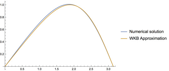
As we can see, the WKB approximation does pretty well in approximating the eigenfunction and doesn't do too bad in estimating the first eigenvalue. However, it is remarkable that even for the first eigenvalue we get such an accurate prediction! After all, the WKB approximation was supposed to only work in the limit that $n\gg1$. Notice also that there are higher order terms that we could've added to the WKB approximation, thus obtaining an even more accurate result for this problem. But it seems that apparently, $n=1$ is close enough to infinity for the asymptotic representation to be a good approximation. As we increase the values of $n$ we get better and better approximations. Now, recall the section on asymptotic matching. Combining this with the power of WKB consists of a tool to further improve our capacity to estimate solutions to differential equations.

#wkb #theory #perturbation #perturbation theory #sturm liouville #pde #ode #odes #mathematics #math #physics #schrodingers cat #schrodinger #equation #quantum mechanics #quantum #yas #problems #solved #solve

[asymptotichigh5]

The magic of $\varepsilon$ (Part II: Asymptotics)

Note of the author: this article was meant to be given the name of this blog.

In physics and probably in other disciplines as well, it is common abuse of notation to use symbols such as $\sim$ or $\ll$. However, we may give a rigorous notion to these symbols in mathematics. For instance we can define two functions $f(x)$ and $g(x)$ to be asymptotic to each other. In that case we can define:$$ f(x) \sim g(x) \text{ as } x \to a \iff \lim_{x \to a} \frac{f(x)}{g(x)} = 1 $$We read $f(x)$ is asymptotic to $g(x)$ as $x$ approaches $a$. As stated above this is n equivalence relation. Furthermore, we might notice that nothing can ever be asymptotic to zero, so we will need to be a little careful when we write things using asymptotics. There are theorems that state that we may differentiate, integrate, subtract, add, multiple, etc. while using asymptotics. In other words, we may perform most of the normal operations we could do with equality, however, exponentiation is an important exception to this. The reason for this will be explained later. In a similar fashion, we may give a concrete definition for $\ll$ as follows:$$ f(x) \ll g(x) \text{ as } x \to a \iff \lim_{x \to a} \frac{f(x)}{g(x)} = 0 $$We read, $f(x)$ is negligible with respect to $g(x)$ as $x \to a$. Now that we have defined the above, we may fully exploit the power of asymptotics.

Asymptotics provides us with a way of estimating a function within a certain limit. Combining this with perturbation theory can yield very powerful results. Normally, we use asymptotics to study the behaviour of functions as they approach infinity or as they approach zero, but it's not always easy to take limits in between. However, we may perform what is called "asymptotic matching" in the transient region in order to get a sense of how the function behaves. For example, consider the differential equation:$$y'(x) + \left(\varepsilon x^2 + 1 + \frac{1}{x^2}\right) y(x) = 0$$We impose boundary conditions $y(1)=1$. 

Notice that this equation is clearly solvable exactly, however the purpose of this example is more to illustrate the method rather than to solve a genuinely difficult problem. In later sections however, when we have built more tools to estimate the asymptotics of differential equations using WKB-theory, we will see that Asymptotic Matching can actually be a great tool. For small $x$, we have that $\varepsilon x^2 \ll 1$ and $\varepsilon x^2 \ll \frac{1}{x^2}$. So we may neglect this term, so then the equation for the "left" $y_L$part becomes:$$ y_L'(x) + \left(1 + \frac{1}{x^2}\right) y_L(x) = 0$$With the same boundary conditions. Solving this equation we have that $y_L(x) = e^{-x+1/x}$. Now let us examine the limit at the "right", that is, when $x$ is large, we have that $\frac{1}{x^2} \ll \varepsilon x^2$ and $\frac{1}{x^2} \ll 1$. We thus have an equation for $y_R(x)$.$$y_R'(x) + (\varepsilon x^2 + 1)y_R(x) =0$$Which again, we may easily solve to obtain $y_R(x) = ae^{-x-\varepsilon x^3/3}$ where $a$ is a constant. Notice however that there is a region where both approximations are valid, namely the region where $e^{-x+1/x} \sim e^{-x}$ and simultaneously requiring $ae^{-x-\varepsilon x^3/3} \sim ae^{-x}$. Notice that in this region, both asymptotic approximations must agree so we have that $a \sim 1$. We can also easily determine that this region corresponds to $1 \ll x \ll 1/\varepsilon^{1/3}$ as $\varepsilon \to 0$. However, this is simply the first order approximation, we can improve the asymptotic matching by considering further terms in the perturbation expansion, this will yield a better result in the transient region.

We proceed as follows: start by considering the original differential equation and plug in the perturbation example for $y(x) = \sum y_n(x) \varepsilon^n$. By doing so, we get a condition on the $y_n(x)$'s. For simplicity, we consider the first order correction only, which yields the condition for $y_1(x)$:$$y_1'(x) + \left(1 + \frac{1}{x^2}\right) y_1(x) = -x^2 y_0(x)$$Now, we have already previously solved for $y_0(x)= e^{-x+1/x}$. Thus we may solve this equation to obtain $y_1(x) = -e^{-x+1/x}\left(\frac{x^3-1}{3}\right)$. So overall, we now have a better approximation for $y_L(x)$, namely:$$y_L(x) = e^{-x+1/x}\left(1+\varepsilon \frac{1-x^3}{3}+O(\varepsilon^2 x^6)\right)$$Using WKB-theory (which we shall explain further on), we may get an asymptotic approximation in the "right" region, namely: $y_R(x) = a e^{-\varepsilon x^3/3 -x +1/x}$. Notice that this is actually the exact solution of the differential equation (simply because WKB theory is that powerful), but assuming that we are in the overlapping region, we may expand this as:$$y_R(x) = a e^{-x+1/x}\left(1-\varepsilon \frac{x^3}{3} + O(\varepsilon^2 x^6)\right)$$Comparing the results for $y_R(x)$ and $y_L(x)$ and considering we are in the overlapping region yields a condition for $a$, namely: $a \sim 1+\varepsilon/3$ as $\varepsilon \to 0$. Notice that this is indeed the first term in the linear approximation as the real value for $a=e^{\varepsilon/3}$. This gives an illustration on to how we should then proceed if we wish to refine our approximations to a problem given two asymptotic expansions.  

Can I get an amen over here?

#perturbation #perturbation theory #asymptotics #approximations #approximately #ish #wing it #but this is serious #important #cool stuff #im such a nerd #mathematics #physics #math #maths #differential equation #differential #asymptote

[asymptotichigh5]

The magic of $\varepsilon$ (Part I)

It is clear that the most interesting problems in many disciplines are often not solved analytically and for the most part, if an analytical solution exists, it has already been discovered. This is an effort to provide the reader with a toolkit to empower him to deal with many of these "hard problems" analytically. Why resort to analytical methods to begin with? Numerical methods can sometimes have quite a bit of issues and blindingly solving a problem numerically does not provide the reader with insight about the problem. On the other hand, the perturbative approach provides us with an analytical tool, free from numerical error that allows us to understand the behaviour of said "hard problems". Another reason is of course: you may obtain a numerical result but, how do you know it's right? You need some kind of analytical way of verifying the solutions that you get out of the computer.

When faced with a "hard problem", the spirit of perturbation theory can be summarized to three simple steps:

Formulate the "hard problem" as a function of a parameter $\varepsilon$

Assume that the answer has a representation in the form of Taylor-like series $\sum_{n=0}^{\infty} a_n \varepsilon^n$

Add up the series

Sounds reasonably simple. But at each of these steps, there are different issues that come up and we shall see how to deal with them (or at least some of the possible details that can be of relevance when solving different types of perturbation problems).

Why does perturbation theory work?

Perturbation theory works wonderfully because it doesn't really solve the problem. At least not exactly. We may get an arbitrarily accurate answer, but never the exact answer. To do this, perturbation theory breaks the difficulty of the original problem into infinitely many "easy" problems. Heuristically, the difficulty of the problem is spread in some way. 

We should probably start to look at the power of perturbation theory with a simple example. Consider solving the diffential equation $$ y''(x) = f(x) y(x) $$ Where we only assume that $f(x)$ is continuous and we will impose boundary conditions $y(0)=1$ and $y'(0)=1$ (one may generalize this in the obvious way). In general, this is an extremely difficult problem that is, in many cases, not solvable analytically. However, solving the problem using a perturbative approach makes this look easy!

Let us start with step number (1) and insert our parameter $\varepsilon$ in. We then have:$$y''(x) = \varepsilon f(x) y(x) $$ Now, notice that when $\varepsilon=0$, we recover our unperturbed problem, which we always will demand to be exactly solvable. In our case, it is a piece of cake: $y_0''(x) = 0$ with the above boundary conditions. This yields the solution: $y_0(x) = 1+x$. Now that we have solved the unperturbed problem, we can apply our ansatz given in step (2) and plug the series back into the differential equation to obtain:$$ \sum_{n=1}^\infty y_n''(x) \varepsilon^n = f(x) \sum_{n=1}^\infty y_{n-1}(x) \varepsilon^{n} $$ Equating powers of $\varepsilon$, we get a recursive relation for the $y_n(x)$'s. Notice that in doing this, we assume that the Taylor series exists and thus we can do this because Taylor series are unique. So we obtain:$$ y_n''(x) = f(x) y_{n-1}(x) $$ Notice that since the boundary conditions are already satisfied by the unperturbed problem, we may impose the following boundary conditions for the rest of of the series: $y_n(0)=0$ and $y_n'(0) = 0$. Then, we may simply integrate the above equation twice to get an explicit answer for $y_n(x)$. $$y_n(x) = \int_0^x dt \int_0^t ds \, y_{n-1}(s) f(s)$$ As an example we can try to solve the following differential equation: $$ y''(x) = -e^{-x} y(x)$$This equation, while very complicated-looking is actually still analytically solvable in terms of Bessel functions:$$y(x)  = \frac{[Y_0(2)+Y_0'(2)]J_0(2e^{-x/2})-[J_0(2)+J'(2)]Y_0(2e^{-x/2})}{J_0(2)Y_0'(2)-J_0(2)Y_0(2)} $$

But, I think everyone agrees that obtaining this solution is a non-trivial feat and a quite challenging deed. However, perturbatively, the problem is a joke! It is reduced to simple old integration by parts. Applying the formula we obtained before, we can get some expressions for the first terms of the perturbation series. The first terms are $y_1(x) = 3-2x-e^{-x}(3+x)$ and $y_2(x) = e^{-2x}(1+e^x(x-1))(3+x+e^x(2x-3))$, etc. 

So how good exactly is this method then? Well, to compare it we can use a very wide-spread method: the Frobenius method of solving differential equations. Now you might initially think that these two approaches are actually very similar due to their infinite series nature, however, perturbation theory is many, many times better.

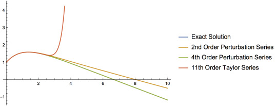
As we can see from the figure, after 11 terms, the Taylor series still does very poorly at converging, even though it is convergent everywhere. On the other hand, after only adding up 4 terms in the perturbation series, we have magnificent accuracy even for high values of $x$. In fact, the error goes like $O(\ln(x))$! The obvious question is why? Why does perturbation theory do so well in comparison to good old Taylor series? The best way to understand this, at least intuitively, is to go to the complex plane. If there is a Taylor series around zero, it must converge up to the next pole, which in the case of some functions can actually be a pretty heavy constraint. Consider for example $\Gamma(z)^{-1}$, this function is actually entire in the complex plane, but exhibits very different behaviour around zero. On the negative real axis, it is oscillating pretty violently while on the positive axis, it is decaying quite quickly. So we can see that if the Taylor series converges everywhere, the poor thing has to mimic the behaviour on both sides. This puts tremendous pressure on the series, hence why it converges so slowly. 

In contrast, you don't really ask that much about a perturbation series in general, you simply demand it to converge on a cut of the complex plane, so it is not so surprising that we get such a dramatic difference in convergence speed. However, for most applications, we only need to know the behaviour of a function in a certain region of the complex plane anyway, which is why perturbative methods are preferable.

#perturbation #perturbation theory #quantum #science #maths #mathematics #mathemagics #yas #yasss #still cool #so cool #awesome #powerful #differential #differential equation #pde

[asymptotichigh5]

Well, math does have sin’s in it... Cos it can

Math jokes aren’t funny. nothing about math is funny. math is a sin

[asymptotichigh5]

On dealing with a large number of degrees of freedom (very mathy)

So I’m supposed to be studying for my statistical thermodynamics exam tomorrow, but I can’t be bothered, so I decided to write about it. In part to feel like I’m doing something that will actually help me on tomorrow’s test I guess. 

We know that thermodynamics is all about “equilibrium” and values of quantities at “equilibrium” and how heat can flow from one place to another and so on and so forth. But what is never really defined properly in any thermodynamics class I’ve ever taken is what equilibrium actually is. Furthermore, it is never explored as to how the system reaches equilibrium, or if it even does indeed reach equilibrium. So we shall start this (probably series) of posts by asking us the following questions. 

How can we define equilibrium?

Do all systems naturally evolve towards an equilibrium state as defined by (1)?

How can we describe the time evolution of a system that is not yet in equilibrium?

Without loss of generality (for now at the very least) let us concentrate our efforts into describing a system like for example the ideal gas. Now I know what you’re thinking, obviously you’d pick a gas. 

And yes, to a certain extent it was obvious. You see a gas, in particular an ideal gas, is the easiest system we can consider and for an introduction, it’s the perfect example of exactly what mathematical methods need to be employed in more complex situations.

To examine the behaviour of the gas, let us consider all the information that is technically available to us from a classical mechanics perspective. We could consider for instance, having a super computer and keeping track of the positions \(\vec{q}_i(t)\) and momenta \(\vec{p}_i(t)\) of all \(N \sim 10^{23}\) particles in our typical gas sample. Of course, there is way too much information and this is exactly why this problem is challenging. However, the equations governing the motion of these particles is actually quite simple. 

Due to classical mechanics, we may describe the time evolution of the system by considering a general Hamiltonian of the system given by $$\mathcal{H}= \sum_{n=1}^{N}\left( \frac{\vec{p}_i^2}{2m}+U(\vec{q}_i) \right) + \sum_{i \neq j} V(|\vec{q}_i-\vec{q}_j|)$$ In principle, \(U(\vec{q}_i)\) is free to be any potential you want and \(V(|\vec{q}_i-\vec{q}_j|)\) is the potential due to the interaction of the particles with each other. 

As you can imagine, dealing with this situation would be very difficult, however for now, let’s see for how long we can get away with the full generality of the situation. We conclude also that nature is a hell of a computer.

Of course, because we are treating this classically, the time evolution of this system is simply given by Hamilton’s equations, which are $$\frac{\partial \vec{q}_i}{\partial t} = \frac{\partial \mathcal{H}}{\partial \vec{p}_i} $$ $$ \frac{\partial \vec{p}_i}{\partial t} = -\frac{\partial \mathcal{H}}{\partial \vec{q}_i} $$ We define a microstate as being a point \(\mu(t)\) in the \(6N\) dimensional space \(\Gamma = \prod_{n=1}^{N} \{q_i,p_i\}\) whose evolution is governed by the equations above. Notice that as usual, the classical mechanics equations of motion exhibit time-reversal symmetry, so they are invariant under the transformation \(T(\mathbb{p},\mathbb{q}) \to (-\mathbb{p},\mathbb{q})\). That is, if we were to reverse all the momenta of all particles \(\mathbb{p}\) at any point in time, the system would simply come back exactly where it originally came from. This observation of course, is counter intuitive, after all in the case of a gas, once it escapes we know intuitively that the gas does not go back into its original container. And making it go back completely is a very difficult task. So another question we can ask ourselves and that we should ask ourselves in the process of the analysis of this system is: at what point will we lose reversibility?

However, for our purposes, we really couldn’t care less if particle 3 has a certain momentum. In some kind of way, we only care about only what the gas does as a whole. So we care about things like pressure, volume, etc. Defined more precisely, we can say that a macrostate \(M\) of the system is uniquely specified by three so-called state functions such as the energy \(E\), the pressure \(P\), etc. So formally it is a triplet of state functions. 

As you can imagine, given any particular macrostate, it must be that more than one microstate corresponds to it. After all, there so many more microstates than macrostates. The only possibility is thus the previous statement. 

Next, we need to perform somewhat of a weird exercise to come up with a good definition. Imagine that I literally copy paste my system and make \(\mathcal{N}\) copies of it (ain’t nobody got time for that, but suppose you did). We then choose a different representative point \(\mu_n(t)\) in the phase space \(\Gamma\) that corresponds to a microstate that describes indeed our macrostate \(M\). Now consider an infinitesimal volume \(d\Gamma = d^{3N}p_i  d^{3N}q_i\) around the point \(\mu(t)\). If we let \(d\mathcal{N}\) denote the number of representative points within this volume \(d\Gamma\) we can define a probability density function:$$ \rho(\mu) d\Gamma = \lim_{\mathcal{N} \to \infty} \frac{d\mathcal{N}}{\mathcal{N}} $$ So fine, we were meticulously careful, which I usually dislike doing in this blog to arrive at this definition and it’s nice and all but asides just writing definitions and babbling, what have we actually accomplished? Well, at least in theory so far we can take averages of things, which is nice, I guess.

But the thing is, we know really nothing about this mysterious phase space to be able to say anything nice about it so far. So we must dwell into venturing in \(6N\) dimensional space for a while, I guess. If you ever needed some room in your life, you’re about to get it.

I usually don’t make comments about gifs, but concerning the above one, you’re probably shooing away or praying to the lord for the formality to be over. I regret to tell you it’s not, which is nice if you’re a mathematician. But you see, formal systems are not always a bad thing. In fact, in my opinion they’re quite nice. They’re clear and the formal definitions of things doesn’t leave ambiguities. Everything is nice and defined which provided a good mathematical background to deal with a hard problem. That is the main goal of this article.

Next let us try to find out more about this \(\Gamma\)-space we have defined. To do this let us consider a tiny step time \(\delta t\) and imagine we are sitting at point \((\mathbb{p},\mathbb{q})\). Thus after this tiny time step, we will land at the point given by coordinates \((\mathbb{p}’,\mathbb{q}’)\) given by: $$ q_{\alpha}’ = q_{\alpha} + \frac{\partial q_{\alpha}}{\partial t}\delta t + O(\delta t^2) $$ $$ p_{\alpha}’ = p_{\alpha} + \frac{\partial p_{\alpha}}{\partial t}\delta t + O(\delta t^2) $$ But then of course, it follows naturally that because our time step is very small order of \(\delta t^2\) is negligible so we can throw it away (this would be rigorous in non-standard analysis, which I will probably talk about in a future article). Furthermore, because we are looking at a hypercube, the distortions of the sides of the cube will depend on the coordinates of the points of the side of the cube, so we can transform our expressions into: $$ q_{\alpha}’ = q_{\alpha} + \frac{\partial^2 q_{\alpha}}{\partial q_{\alpha} \partial t}dq_{\alpha}\delta t + O(\delta t^2) $$ $$ p_{\alpha}’ = p_{\alpha} + \frac{\partial^2 p_{\alpha}}{\partial p_{\alpha} \partial t}dp_{\alpha}\delta t + O(\delta t^2) $$ Now notice that the new volume of the distorted infinitesimal hypercube is simply the infinitesimals of \(\mathbb{p}’\) and \(\mathbb{q}’\) multiplied so we have $$ dq_{\alpha}’ dp_{\alpha}’ = dq_{\alpha} dp_{\alpha} \left[ 1 + \left( \frac{\partial^2 q_{\alpha}}{\partial q_{\alpha} \partial t}dq_{\alpha} +\frac{\partial^2 p_{\alpha}}{\partial p_{\alpha} \partial t}dp_{\alpha} \right) \delta t + O(\delta t^2) \right] $$ Now we make use of Hamilton’s equations to get rid of the time derivative and swap it for a momentum or position one respectively and we simply obtain: $$dq_{\alpha}’ dp_{\alpha}’ = dq_{\alpha} dp_{\alpha} \left[ 1 + \left( \frac{\partial^2 q_{\alpha}}{\partial q_{\alpha} \partial p_{\alpha}}dq_{\alpha} - \frac{\partial^2 p_{\alpha}}{\partial p_{\alpha} \partial q_{\alpha}}dp_{\alpha} \right) \delta t + O(\delta t^2) \right] =dq_{\alpha} dp_{\alpha} $$

Thus we have that up to this order of \(\delta t\), our phase space remains the same in volume. In some kind of way, we can thus think of it as an incompressible volume. Now notice that this theorem we just proved holds in all generality for any Hamiltonian set of equations. In no way did we invoke the ideal gas specifically. 

But this incompressibility condition now gives us the tools to say something more about our probability density function that we previously defined. However, I think I have tortured you with enough math in one post. The next one will probably be a bit lighter, but nonetheless, the rigour is important, because what we are doing is laying the foundations for our understanding of thermodynamics, thus, we have no choice but to have this level of rigour and consistency.

#thermo #thermodynamics #liouville #french #thermodynamic #physics #phase #space #dimensions #calculus #maths #rigorous #OMG #tedious