#model1 | Explore Tumblr Posts and Blogs

sirenlulls · 7 months

Text

bad idea, right? → theburntchip

pairing , theburntchip x youtuber!reader

summary , where the much-mourned couple of the uk youtube scene reconnect

note , this is in aid of my wifey @whoetoshaw who sends the chip lovers in her inbox my way 🤭🫶

part two (get him back!)

yes, i know that he’s my ex, but can’t two people reconnect?!

[tagged: ynapparel , model1 , model2 , model3]

❤️ liked by theburntchip, freyanightingale, and 92,787 others

yourusername EEEE!!!! so happy to announce the launch of my clothing brand, y/n apparel (so original ik 😩💋) the official site will launch on the 21st of september & will bring you a wide variety of styles, from loungewear, to club dresses, to athleisure. i’ve been working on this for little over two and a half years now with my beautiful, creative, incredible, and innovative team. i love love love u all my fashion family @ ynapparel. and i love U!!!! for supporting me 🫶💗 looking forward to seeing u on the apparel account’s insta live as we greet and interview your fav influencers at the launch party x 🥰🥰

user the post hasn’t even been up a minute and chip liked ☹️😭

faithlouisak so so proud of you my babe. actually bawling 🥹🥹

yourusername luv u sm beautiful mama 🫶🫶🫶

thefellasstudios ayyyy! we better see some fire fits on the 21st 😮‍💨

calfreezy now i’m off the professional account, so proud and let’s hope you still remember how to throw a party because i cannot be seen at a stinker

yourusername won’t let u down calfreezy sir 🫡

taliamar baby’s all grown up 🥺 so proud of you my love i can’t wait to see the art you make 🫶

user talia are you crying be honest

georgeclarkeey can you get me a stylist i’m scared to be judged

yourusername i’ll get u set up in a gorg pink bodycon x

maxbalegde @ yourusername i reckon he’d pull it off

maxbalegde THATS MY GIRL!!! 😭😭😭 buzzing for you babes xx

gkbarry_ UGH! i’ll bawl i’m so proud of u girl ❤️

bambinobecky better be seeing you fashion week 2024

yourusername go big or go home ig 🤷‍♀️

user i wanna buy to support but i’m broke so what are the prices gonna be like?

yourusername me and the team tried to keep prices as low as possible but to make sure we were using ethical and durable means of production, we have to keep them pretty middle-ground. around £35/50 quid for the dresses but everything else is pretty diverse in price 💗

user just in time for me to get my winter wardrobe 🤭🥰

model2 loved working with you!! you’re such an angel 💗

yourusername awh my stunning girl!! you’re the sweetest thing & i look forward to working with you again 🫶🫶

[tagged: ynapparel , arthurtv , freyanightingale , zerkaa , gkbarry_ , faithlouisak , calfreezy , chrismd , stephentries , theobaker]

❤️ liked by geenelly, angryginge13, and 97,863 others

yourusername so so so honoured to have the chance to spend a night celebrating my passion project with the people i care the most about. i love u all a million more times than u could ever know. (ft. some very distinguished, very sloshed gentlemen in the last two slides 🥰)

ksi 🖤🔥

freynightingale that pic omg i’ll cry 😭 it was such an amazing night for such an amazing brand and such an amazing woman!! you deserve all the greatness you get ❤️❤️❤️

user mother is motheringgggggg

ynapparel 🩷🩷🩷

gkbarry_ you looked so gorg babe i wanted to take a bite out of you x

yourusername who’s saying you can’t 😩😩

stephentries you know it’s a good night when chrisMD gets his tits out

user losing my mind ur so beautiful

calfreezy NAHHH WHY DID YOU DO THEO LIKE THAT

miaxmon had an absolute ball!!! you looked incredible babe 🫶💋

arthurnfhill it was all fun and games until the karaoke came out to play

yourusername pretending it didn’t happen

user THEY INTERVIEWED CHIP ON THE IG LIVE

user OMG WHY DID HE SAY

user he looked like he was tryna keep it brief but he said he was so proud of y/n because he’s seen how hard she’s worked for this & she deserves it all 🥹🥹🥹 & he also called cal a bellend because he crashed the interview by slapping chip’s bum

[tagged: theburntchip]

❤️ liked by wroetoshaw, willne, and 1,021,363 others

yourusername can’t two people reconnect?

comments on this post have been restricted.

481 notes · View notes

cashmonei · 1 year

Text

Turning ur ultrakill ocs into flight rising dragons is NOT selfcare this shit is so fucking hard WHY IS THE DRESSING ROOM SO SHIT AUGHH.

Anyways. M1-SUPPLY (Model1-SUPPLY)/M1 the beloved. They're fuelled by thermal heat and also sulfur teehee

#fox screeches #i like my ocs and i am gonna talk abt them more ithink

5 notes · View notes

viianey-gutma · 7 days

Text

Data Analysis Tools

The final task deals with testing a potential moderator. By testing a potential moderator, which makes us wonder if there is an association between two constructs for different subgroups within the sample.

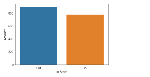
The data set contains variables about purchases in some regions, to determine whether any age group purchases more in-store or out-of-store.

Qualitative variables: In.Store, region Quantitative variables: Age, Amount, items

Python code

import pandas as pd import statsmodels.formula.api as smf import seaborn import matplotlib.pyplot as plt

def ageGroup(row): if row["age"]>60: return "Senior " elif row["age"]>30: return "Adult" elif row["age"]>=18: return "Young" elif row["age"]>9: return "Teenage" else: return "Child"

data = pd.read_csv('Demographic_Data_Orig.csv', low_memory=False)

data['age'] = data['age'].apply(pd.to_numeric, errors='coerce') data['items'] = data['items'].apply(pd.to_numeric, errors='coerce') data['amount'] = data['amount'].apply(pd.to_numeric, errors='coerce')

data["AgeGroup"]=data.apply(ageGroup, axis=1)

data = data[["region","items","in.store","amount", "AgeGroup"]].dropna()

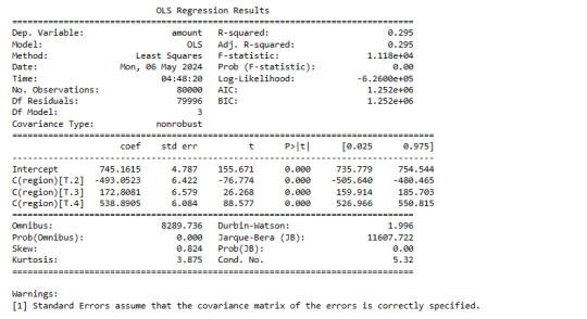
model1 = smf.ols(formula='amount ~ C(region)', data=data).fit() print (model1.summary())

recode1 = {1: 'In', 0: 'Out'} data['in.store']= data['in.store'].map(recode1)

sub1 = data[['amount', 'in.store']].dropna()

print ("means for Amount by Region") m1= sub1.groupby('in.store').mean() print (m1)

print ("standard deviation for mean Amount by In vs Out Store") st1= sub1.groupby('in.store').std() print (st1)

seaborn.barplot(x="in.store", y="amount", data=data, ci=None) plt.xlabel('In Store') plt.ylabel('Amount')

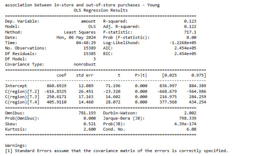
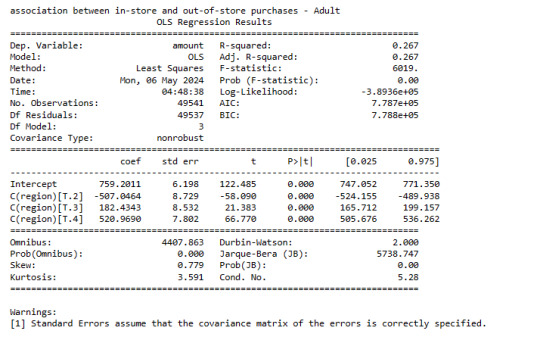
sub2=data[(data['AgeGroup']=='Young')] sub3=data[(data['AgeGroup']=='Adult')] print ('association between in-store and out-of-store purchases - Young') model2 = smf.ols(formula='amount ~ C(region)', data=sub2).fit() print (model2.summary())

print ('association between in-store and out-of-store purchases - Adult') model3 = smf.ols(formula='amount ~ C(region)', data=sub3).fit() print (model3.summary())

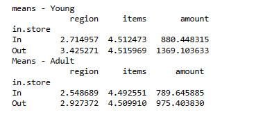
print ("means - Young") m3= sub2.groupby('in.store').mean() print (m3) print ("Means - Adult") m4 = sub3.groupby('in.store').mean() print (m4)

General Result

Young Group

Adult Group

Mean

0 notes

crazygadgetshere · 11 days

Text

Hobbyboss released the RMS Olympic & Nuclear 'East Wind' in June

In our preview, we look at the colours, decals & build up kits. We look at the colours, decals & build up kits in our preview… Preview: The RMS Olympic & Nuclear “East Wind” from Hobbyboss in June RMS Olympic by Hobby Boss : 83421 Model1/700th scale RMS Olympic was a British ocean liner and the lead ship of the White Star Line’s trio of Olympic-class liners. Olympic’s career was 24 years long,…

View On WordPress

0 notes

colorholicsmarketplace · 2 months

Text

Ultra-thin flipper cabinet is light luxury and space-saving, 17cm household entrance entrance cabinet, modern and simple small apartment storage

https://cloud.video.taobao.com/play/u/2217131934901/p/2/e/6/t/1/446029422716.mp4 Product attributes MaterialArtificial board Item numberAL styleSimple and modern Processing methodsSample customization brandother model1 Specifications support image uploadyes Specificationsuit color0.6m + ultra-thin rock slab 17cm without stool, 0.6m + ultra-thin rock slab 24cm without…

View On WordPress

0 notes

pepilagares · 3 months

Video

youtube

Priscilla Ricart Top Model1

#youtube

0 notes

dianaventuresl · 4 months

Video

flickr

♫ I've never seen you shine so bright, you were amazing por ♎︎ Iηαηηα Beauty ♎︎ Via Flickr: ♫ youtu.be/XrAV4rYGCQQ?si=bYL_USA-faFcRkyg ♥♥ Model1 (Diana) ✔Earrings : RAWR! Paradox HUMAN FEMALE EvoX Earrings - @Mainstore ✔Necklace : RAWR! Paradox Necklaces - @Mainstore ✔Armlets: RAWR! Paradox Armlets - @Mainstore ✔Bracelets: RAWR! Paradox Bracelets - @Mainstore ✔Rings: RAWR! Paradox Rings - @Mainstore ✔Garter: RAWR! Paradox Garters - @Mainstore ✔Dress: Virtual Diva Couture - Pasion Dress (Carmin) - @Mainstore ✔Pose : [..::CuCa::..] New Year FF 01 Bento Couple Pose - @Mainstore ♥♥ Model2 (Liss) Thx my friend ♥ ✔Dress: Virtual Diva Couture - Pasion Dress (Crow)- @Mainstore

#rawr #pasion #slvirtual #girlvirtual #virtual #virtualdiva #virtualdivacouture #virtualgirl #dress #collab #friends #flickr

0 notes

theanalyst92 · 4 months

Text

Data analysis tools | week 1

import numpy import pandas import statsmodels.formula.api as smf import statsmodels.stats.multicomp as multi

data = pandas.read_csv('nesarc.csv', low_memory=False)

setting variables you will be working with to numeric

data['S3AQ3B1'] = pandas.to_numeric(data['S3AQ3B1'])

data['S3AQ3B1'] = data['S3AQ3B1'].convert_objects(convert_numeric=True)

data['S3AQ3C1'] = data['S3AQ3C1'].convert_objects(convert_numeric=True)

data['S3AQ3C1'] = pandas.to_numeric(data['S3AQ3C1'])

data['CHECK321'] = data['CHECK321'].convert_objects(convert_numeric=True)

data['CHECK321'] = pandas.to_numeric(data['CHECK321'])

subset data to young adults age 18 to 25 who have smoked in the past 12 months

sub1=data[(data['AGE']>=18) & (data['AGE']<=25) & (data['CHECK321']==1)]

SETTING MISSING DATA

sub1['S3AQ3B1']=sub1['S3AQ3B1'].replace(9, numpy.nan) sub1['S3AQ3C1']=sub1['S3AQ3C1'].replace(99, numpy.nan)

recoding number of days smoked in the past month

recode1 = {1: 30, 2: 22, 3: 14, 4: 5, 5: 2.5, 6: 1} sub1['USFREQMO']= sub1['S3AQ3B1'].map(recode1)

converting new variable USFREQMMO to numeric

sub1['USFREQMO']= sub1['USFREQMO'].convert_objects(convert_numeric=True)

sub1['USFREQMO']=pandas.to_numeric(sub1['USFREQMO'])

Creating a secondary variable multiplying the days smoked/month and the number of cig/per day

sub1['NUMCIGMO_EST']=sub1['USFREQMO'] * sub1['S3AQ3C1']

sub1['NUMCIGMO_EST']= sub1['NUMCIGMO_EST'].convert_objects(convert_numeric=True)

sub1['NUMCIGMO_EST'] = pandas.to_numeric(sub1['NUMCIGMO_EST'])

ct1 = sub1.groupby('NUMCIGMO_EST').size() print (ct1)

using ols function for calculating the F-statistic and associated p value

model1 = smf.ols(formula='NUMCIGMO_EST ~ C(MAJORDEPLIFE)', data=sub1) results1 = model1.fit() print (results1.summary())

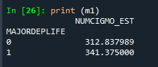
sub2 = sub1[['NUMCIGMO_EST', 'MAJORDEPLIFE']].dropna()

print ('means for numcigmo_est by major depression status') m1= sub2.groupby('MAJORDEPLIFE').mean() print (m1)

_____________________________________

Difference between those two categories is significant. That mean alternative hypothesis is reached.

0 notes

usfstatstudent · 7 months

Text

Module 10 Assignment

library(base) library(ISwR) cystfibr attach(cystfibr) linearmodel <- lm(pemax ~ age + weight + bmp + fev1, data = cystfibr) summary(linearmodel) anova(linearmodel) anovamodel <- aov(pemax ~ age + weight + bmp + fev1, data = cystfibr) summary(anovamodel)

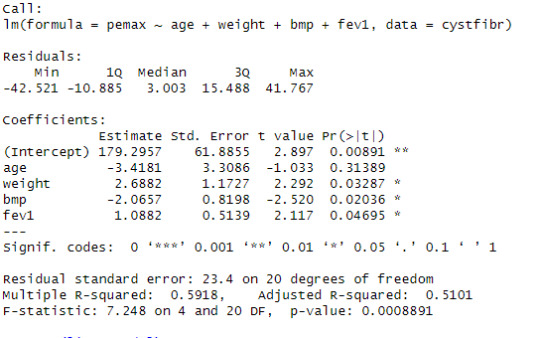
Looking at the linear progression model, we can see that the estimate of the value for the intercept is 179.2957 with significant p-value. The estimate of the variable age is -3.4181 for that unit change in the variable age in the dependent variable pemax with a non-significant p-value. The estimate of the variable weight is 2.6882 for that unit change in the variable weight in the dependent variable pemax with a significant p-value. The estimate of the variable bmp is -2.0657 for that unit change in the variable bmp in the dependent variable pemax with a significant p-value. The estimate of the variable fev1 is 1.0882 for that unit change in the variable fev1 in the dependent variable pemax with a significant p-value.

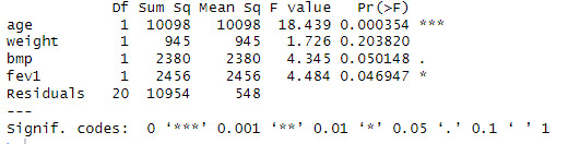
Looking at the ANOVA table, see that the p value of age is 0.00354, less than 0.001 so, we can reject the null hypothesis and can interpret it as the variation the effect of the variable age on the dependent variable pemex is not equal to zero. The p value of weight is 0.203820, greater than 0.05 so, we can not reject the null hypothesis and can interpret it as the variation the effect of the variable weight on the dependent variable pemex is equal to zero. The p value of bmp is 0.050148, less than or equal to 0.05 so, we can reject the null hypothesis and can interpret it as the variation the effect of the variable bmp on the dependent variable pemex is not equal to zero. The p value of fev1 is 0.046947, less than or equal to 0.05 so, we can reject the null hypothesis and can interpret it as the variation the effect of the variable fev1 on the dependent variable pemex is not equal to zero.

Importing Data

library(ISwR) Data <- secher head(Data)

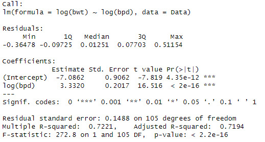
Creating a model using birthweight and biparietal diameter

model1 <- lm(log(bwt) ~ log(bpd) , data = Data) summary(model1)

Creating a model using birthweight and abdominal diameter

model2 <- lm(log(bwt) ~ log(ad), data = Data) summary(model2)

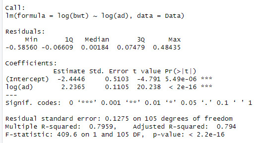
When looking at the data, we can see that the log(bpd) is a significant variable of the log(ad). The model also explains 79.5% of the variation in log(bwt)

Creating a model using birthweight and both abdominal and biparietal diameter

model3 <- lm(log(bwt) ~ log(ad) + log(bpd), data = Data) summary(model3)

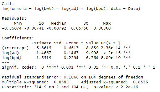
We can see that when both variables are added that the significance and Rsqaured increases to 85.5%.

The interpretation is, when there is a 1% increase in abdominal diameter increases the birthweight by 1.4667% and when there is a 1% increases in the biparietal diameter there is a 1.5519% increase in the birthweight.

0 notes

acacheng · 7 months

Text

running an analysis of variance

import numpy as np import pandas as pd import statsmodels.formula.api as smf import statsmodels.stats.multicomp as multi import matplotlib.pyplot as plt import seaborn as sns

Load data

data = pd.read_csv('nesarc.csv', low_memory=False)

Convert columns to numeric

data['S3AQ3B1'] = pd.to_numeric(data['S3AQ3B1'], errors='coerce') data['S3AQ3C1'] = pd.to_numeric(data['S3AQ3C1'], errors='coerce') data['CHECK321'] = pd.to_numeric(data['CHECK321'], errors='coerce')

Subset data

sub1 = data[(data['AGE'] >= 18) & (data['AGE'] <= 25) & (data['CHECK321'] == 1)].copy()

Replace missing data

sub1['S3AQ3B1'] = sub1['S3AQ3B1'].replace(9, np.nan) sub1['S3AQ3C1'] = sub1['S3AQ3C1'].replace(99, np.nan)

Recode data

recode1 = {1: 30, 2: 22, 3: 14, 4: 5, 5: 2.5, 6: 1} sub1['USFREQMO'] = sub1['S3AQ3B1'].map(recode1)

Convert new variable to numeric

sub1['USFREQMO'] = pd.to_numeric(sub1['USFREQMO'], errors='coerce')

Create secondary variable

sub1['NUMCIGMO_EST'] = sub1['USFREQMO'] * sub1['S3AQ3C1'] sub1['NUMCIGMO_EST'] = pd.to_numeric(sub1['NUMCIGMO_EST'], errors='coerce')

Display group size

ct1 = sub1.groupby('NUMCIGMO_EST').size() print(ct1)

Perform OLS regression for ANOVA

model1 = smf.ols(formula='NUMCIGMO_EST ~ C(MAJORDEPLIFE)', data=sub1).fit() print(model1.summary())

Display means & standard deviations for major depression status

sub2 = sub1[['NUMCIGMO_EST', 'MAJORDEPLIFE']].dropna() print('Means for numcigmo_est by major depression status') print(sub2.groupby('MAJORDEPLIFE').mean()) print('Standard deviations for numcigmo_est by major depression status') print(sub2.groupby('MAJORDEPLIFE').std())

Perform OLS regression for ANOVA with ETHRACE2A

sub3 = sub1[['NUMCIGMO_EST', 'ETHRACE2A']].dropna() model2 = smf.ols(formula='NUMCIGMO_EST ~ C(ETHRACE2A)', data=sub3).fit() print(model2.summary())

Display means & standard deviations for ETHRACE2A

print('Means for numcigmo_est by ETHRACE2A') print(sub3.groupby('ETHRACE2A').mean()) print('Standard deviations for numcigmo_est by ETHRACE2A') print(sub3.groupby('ETHRACE2A').std())

Multi-comparison post-hoc test

mc1 = multi.MultiComparison(sub3['NUMCIGMO_EST'], sub3['ETHRACE2A']) res1 = mc1.tukeyhsd() print(res1.summary())

1 note · View note

worldtourtraveller · 7 months

Text

Week 3 - Generating a Correlation Coefficient

Create a blog entry where you submit syntax used to generate a correlation coefficient (copied and pasted from your program) along with corresponding output and a few sentences of interpretation.

Generate a correlation coefficient. Note 1: Two 3+ level categorical variables can be used to generate a correlation coefficient if the the categories are ordered and the average (i.e. mean) can be interpreted. The scatter plot on the other hand will not be useful. In general the scatterplot is not useful for discrete variables (i.e. those that take on a limited number of values). Note 2: When we square r, it tells us what proportion of the variability in one variable is described by variation in the second variable (a.k.a. RSquared or Coefficient of Determination).

# coding: utf-8

# coding utf-8 # created by Nick Apr 2016

# magic to show charts in notebook get_ipython().magic('matplotlib inline')

# imports import pandas as pd import numpy as np import seaborn as sns import matplotlib.pyplot as plt import statsmodels.formula.api as smf import statsmodels.stats.multicomp as multi

# get data data = pd.read_csv('gapminder.csv', low_memory = False) #print(data.head(5))

# create subset of data containing only columns of interest sub1 = data[['country','femaleemployrate','suicideper100th','employrate']].dropna() #print(sub1.head(30))

# Change str columns to numeric and blanks etc to NaN colsToConvert = ['femaleemployrate','suicideper100th','employrate'] for col in colsToConvert: sub1[col] = pd.to_numeric(sub1[col],errors = 'coerce')

# drop rows where 'suicide' and employment rates are missing sub1 = sub1[pd.notnull(data['suicideper100th'])] sub1 = sub1[pd.notnull(data['femaleemployrate'])] sub1 = sub1[pd.notnull(data['employrate'])]

# I want to convert suicides per 100,00 to suicides per million sub1['suicide'] = sub1['suicideper100th']*10 #print(sub1.head(30))

# drop rows where 'suicide' and employment rates are missing sub1 = sub1[pd.notnull(sub1['suicide'])] sub1 = sub1[pd.notnull(sub1['femaleemployrate'])] sub1 = sub1[pd.notnull(sub1['employrate'])]

# create a categorical variable for suicide rates myBins = [0,29,59,89,119,149,179,209,239,269,299,329,360] myLabs = ['0-29','30-59','60-89','90-119','120-149','150-179','180-209','210-239','240-269','270-299','300-329','330-360'] sub1['suicideCat']= pd.cut(sub1.suicide, bins = myBins, labels = myLabs) #print(sub1.head(30))

# create a categorical variable for suicide rates print(sub1['employrate'].describe()) myBins = [34,43,55,65,74,84] myLabs = ['Very Low','Low','Mid Range','High','VeryHigh'] sub1['TotEmpRate']= pd.cut(sub1.employrate, bins = myBins, labels = myLabs) # print(sub1.head(30))

# using ols function for calculating the F-statistic and associated p value model1 = smf.ols(formula='suicide ~ C(TotEmpRate)', data=sub1) results1 = model1.fit() print (results1.summary())

#Lets work out some grouped means on a subset containing only these two columns sub2 = sub1[['suicide','TotEmpRate']].dropna() # sub2['suicide'] = pd.to_numeric(sub2['suicide'],errors = 'coerce') print ('\n','means for suicide by employment rate') m1= sub2.groupby('TotEmpRate').mean() print (m1)

print ('\n\n','standard deviations for suicide by employment rate') sd1 = sub2.groupby('TotEmpRate').std() print (sd1) # print(sub2.head(10)) # print('\n',type(sub2.suicide))

print('Tukey multi comparison of suicides by employment rates','\n') mc1 = multi.MultiComparison(sub2['suicide'], sub2['TotEmpRate']) res1 = mc1.tukeyhsd() print(res1.summary())

# Create a boxplot of the two features sns.boxplot(y = 'suicide', x = 'TotEmpRate', data=sub2)

0 notes

data-science-noob · 8 months

Text

"Comprehensive Data Analysis and Statistical Exploration Script"

The provided Python script is designed for data analysis and statistical processing. It imports and analyzes various datasets, performing statistical tests like ANOVA and linear regression. The script also creates data visualizations and handles data cleaning and transformation tasks.

ANOVA

import numpy import pandas import statsmodels.formula.api as smf import statsmodels.stats.multicomp as multi import seaborn import matplotlib.pyplot as plt

data = pandas.read_csv('diet_exercise.csv', low_memory=False)

data["Diet"] = data["Diet"].astype('category')

data['WeightLoss']= data['WeightLoss'].convert_objects(convert_numeric=True)

d`ir(smf)

model1 = smf.ols(formula='WeightLoss ~ C(Diet)', data=data).fit() print (model1.summary())

sub1 = data[['WeightLoss', 'Diet']].dropna()

print ("means for WeightLoss by Diet A vs. B") m1= sub1.groupby('Diet').mean() print (m1)

print ("standard deviation for mean WeightLoss by Diet A vs. B") st1= sub1.groupby('Diet').std() print (st1)

bivariate bar graph

seaborn.factorplot(x="Diet", y="WeightLoss", data=data, kind="bar", ci=None) plt.xlabel('Diet Type') plt.ylabel('Mean Weight Loss in pounds')

sub2=data[(data['Exercise']=='Cardio')] sub3=data[(data['Exercise']=='Weights')]

print ('association between diet and weight loss for those using Cardio exercise') model2 = smf.ols(formula='WeightLoss ~ C(Diet)', data=sub2).fit() print (model2.summary())

print ('association between diet and weight loss for those using Weights exercise') model3 = smf.ols(formula='WeightLoss ~ C(Diet)', data=sub3).fit() print (model3.summary())

print ("means for WeightLoss by Diet A vs. B for CARDIO") m3= sub2.groupby('Diet').mean() print (m3) print ("Means for WeightLoss by Diet A vs. B for WEIGHTS") m4 = sub3.groupby('Diet').mean() print (m4)

End of Lesson 2

Beginning of Lesson 3

subset data to young adults age 18 to 25 who have smoked in the past 12 months

sub1=data[(data['AGE']>=18) & (data['AGE']<=25) & (data['CHECK321']==1)]

SETTING MISSING DATA

sub1['S3AQ3B1']=sub1['S3AQ3B1'].replace(9, numpy.nan) sub1['S3AQ3C1']=sub1['S3AQ3C1'].replace(99, numpy.nan)

recoding number of days smoked in the past month

recode1 = {1: 30, 2: 22, 3: 14, 4: 5, 5: 2.5, 6: 1} sub1['USFREQMO']= sub1['S3AQ3B1'].map(recode1)

converting new variable USFREQMMO to numeric

sub1['USFREQMO']= sub1['USFREQMO'].convert_objects(convert_numeric=True)

Creating a secondary variable multiplying the days smoked/month and the number of cig/per day

sub1['NUMCIGMO_EST']=sub1['USFREQMO'] * sub1['S3AQ3C1']

sub1['NUMCIGMO_EST']= sub1['NUMCIGMO_EST'].convert_objects(convert_numeric=True)

ct1= sub1.groupby('NUMCIGMO_EST').size() print (ct1)

model1 = smf.ols(formula='NUMCIGMO_EST ~ MAJORDEPLIFE', data=sub1).fit() print (model1.summary())

sub2 = sub1[['NUMCIGMO_EST', 'MAJORDEPLIFE']].dropna()

print ('means for numcigmo_est by major depression status') m1= sub2.groupby('MAJORDEPLIFE').mean() print (m1)

print ('standard deviations for numcigmo_est by major depression status') sd1 = sub2.groupby('MAJORDEPLIFE').std() print (sd1)

sub3 = sub1[['NUMCIGMO_EST', 'ETHRACE2A']].dropna()

model1 = smf.ols(formula='NUMCIGMO_EST ~ C(ETHRACE2A)', data=sub3).fit() print (model1.summary())

print ('means for numcigmo_est by major depression status') m2= sub3.groupby('ETHRACE2A').mean() print (m2)

print ('standard deviations for numcigmo_est by major depression status') sd2 = sub3.groupby('ETHRACE2A').std() print (sd2)

mc2 = multi.MultiComparison(sub3['NUMCIGMO_EST'], sub3['ETHRACE2A']) res2 = mc2.tukeyhsd() print(res2.summary())

CHISQ

import pandas import numpy import scipy.stats import seaborn import matplotlib.pyplot as plt import statsmodels.stats.proportion as sm

data = pandas.read_csv('nesarc_pds.csv', low_memory=False)

setting variables you will be working with to numeric

data['TAB12MDX'] = data['TAB12MDX'].convert_objects(convert_numeric=True) data['CHECK321'] = data['CHECK321'].convert_objects(convert_numeric=True) data['S3AQ3B1'] = data['S3AQ3B1'].convert_objects(convert_numeric=True) data['S3AQ3C1'] = data['S3AQ3C1'].convert_objects(convert_numeric=True) data['AGE'] = data['AGE'].convert_objects(convert_numeric=True)

subset data to young adults age 18 to 25 who have smoked in the past 12 months

sub1=data[(data['AGE']>=18) & (data['AGE']<=25) & (data['CHECK321']==1)]

make a copy of my new subsetted data

sub2 = sub1.copy()

recode missing values to python missing (NaN)

sub2['S3AQ3B1']=sub2['S3AQ3B1'].replace(9, numpy.nan) sub2['S3AQ3C1']=sub2['S3AQ3C1'].replace(99, numpy.nan)

START RUNNING CODE HERE

recoding values for S3AQ3B1 into a new variable, USFREQMO

recode1 = {1: 30, 2: 22, 3: 14, 4: 6, 5: 2.5, 6: 1} sub2['USFREQMO']= sub2['S3AQ3B1'].map(recode1)

recoding values for S3AQ3B1 into a new variable, USFREQMO

recode2 = {1: 30, 2: 22, 3: 14, 4: 5, 5: 2.5, 6: 1} sub2['USFREQMO']= sub2['S3AQ3B1'].map(recode2)

def USQUAN (row): if row['S3AQ3B1'] != 1: return 0 elif row['S3AQ3C1'] <= 5 : return 3 elif row['S3AQ3C1'] <=10: return 8 elif row['S3AQ3C1'] <= 15: return 13 elif row['S3AQ3C1'] <= 20: return 18 elif row['S3AQ3C1'] > 20: return 37 sub2['USQUAN'] = sub2.apply (lambda row: USQUAN (row),axis=1)

c5 = sub2['USQUAN'].value_counts(sort=False, dropna=True) print(c5)

c6 = sub2['S3AQ3C1'].value_counts(sort=False, dropna=True) print(c6)

contingency table of observed counts

ct1=pandas.crosstab(sub2['TAB12MDX'], sub2['USQUAN']) print (ct1)

column percentages

colsum=ct1.sum(axis=0) colpct=ct1/colsum print(colpct)

chi-square

print ('chi-square value, p value, expected counts') cs1= scipy.stats.chi2_contingency(ct1) print (cs1)

set variable types

sub2["USQUAN"] = sub2["USQUAN"].astype('category') sub2['TAB12MDX'] = sub2['TAB12MDX'].convert_objects(convert_numeric=True)

bivariate bar graph

seaborn.factorplot(x="USQUAN", y="TAB12MDX", data=sub2, kind="bar", ci=None) plt.xlabel('number of cigarettes smoked per day') plt.ylabel('Proportion Nicotine Dependent')

sub3=sub2[(sub2['MAJORDEPLIFE']== 0)] sub4=sub2[(sub2['MAJORDEPLIFE']== 1)]

print ('association between smoking quantity and nicotine dependence for those W/O deperession')

contingency table of observed counts

ct2=pandas.crosstab(sub3['TAB12MDX'], sub3['USQUAN']) print (ct2)

column percentages

colsum=ct1.sum(axis=0) colpct=ct1/colsum print(colpct)

chi-square

print ('chi-square value, p value, expected counts') cs2= scipy.stats.chi2_contingency(ct2) print (cs2)

print ('association between smoking quantity and nicotine dependence for those WITH depression')

contingency table of observed counts

ct3=pandas.crosstab(sub4['TAB12MDX'], sub4['USQUAN']) print (ct3)

column percentages

colsum=ct1.sum(axis=0) colpct=ct1/colsum print(colpct)

chi-square

print ('chi-square value, p value, expected counts') cs3= scipy.stats.chi2_contingency(ct3) print (cs3)

seaborn.factorplot(x="USQUAN", y="TAB12MDX", data=sub4, kind="point", ci=None) plt.xlabel('number of cigarettes smoked per day') plt.ylabel('Proportion Nicotine Dependent') plt.title('association between smoking quantity and nicotine dependence for those WITH depression')

seaborn.factorplot(x="USQUAN", y="TAB12MDX", data=sub3, kind="point", ci=None) plt.xlabel('number of cigarettes smoked per day') plt.ylabel('Proportion Nicotine Dependent') plt.title('association between smoking quantity and nicotine dependence for those WITHOUT depression')

End of Lesson 3

Beginning of Lesson 4

CORRELATION

import pandas import numpy import scipy.stats import seaborn import matplotlib.pyplot as plt

data = pandas.read_csv('gapminder.csv', low_memory=False)

data['urbanrate'] = data['urbanrate'].convert_objects(convert_numeric=True) data['incomeperperson'] = data['incomeperperson'].convert_objects(convert_numeric=True) data['internetuserate'] = data['internetuserate'].convert_objects(convert_numeric=True) data['incomeperperson']=data['incomeperperson'].replace(' ', numpy.nan)

data_clean=data.dropna()

print (scipy.stats.pearsonr(data_clean['urbanrate'], data_clean['internetuserate']))

def incomegrp (row): if row['incomeperperson'] <= 744.239: return 1 elif row['incomeperperson'] <= 9425.326 : return 2 elif row['incomeperperson'] > 9425.326: return 3

data_clean['incomegrp'] = data_clean.apply (lambda row: incomegrp (row),axis=1)

chk1 = data_clean['incomegrp'].value_counts(sort=False, dropna=False) print(chk1)

sub1=data_clean[(data_clean['incomegrp']== 1)] sub2=data_clean[(data_clean['incomegrp']== 2)] sub3=data_clean[(data_clean['incomegrp']== 3)]

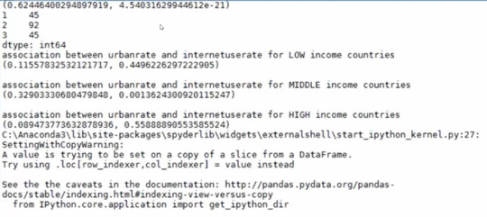
print ('association between urbanrate and internetuserate for LOW income countries') print (scipy.stats.pearsonr(sub1['urbanrate'], sub1['internetuserate'])) print (' ') print ('association between urbanrate and internetuserate for MIDDLE income countries') print (scipy.stats.pearsonr(sub2['urbanrate'], sub2['internetuserate'])) print (' ') print ('association between urbanrate and internetuserate for HIGH income countries') print (scipy.stats.pearsonr(sub3['urbanrate'], sub3['internetuserate']))

scat1 = seaborn.regplot(x="urbanrate", y="internetuserate", data=sub1) plt.xlabel('Urban Rate') plt.ylabel('Internet Use Rate') plt.title('Scatterplot for the Association Between Urban Rate and Internet Use Rate for LOW income countries') print (scat1)

scat2 = seaborn.regplot(x="urbanrate", y="internetuserate", fit_reg=False, data=sub2) plt.xlabel('Urban Rate') plt.ylabel('Internet Use Rate') plt.title('Scatterplot for the Association Between Urban Rate and Internet Use Rate for MIDDLE income countries') print (scat2)

scat3 = seaborn.regplot(x="urbanrate", y="internetuserate", data=sub3) plt.xlabel('Urban Rate') plt.ylabel('Internet Use Rate') plt.title('Scatterplot for the Association Between Urban Rate and Internet Use Rate for HIGH income countries') print (scat3)

0 notes