usfstatstudent

[usfstatstudent]

Final project

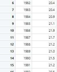
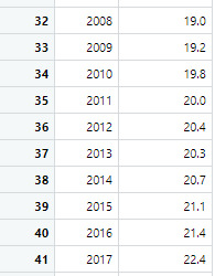
Topic: Death rates for suicide, by sex, race, Hispanic origin, and age: United States

For my final project, I wanted to do something that I thought was important. As the topic of mental health issues continue to become a more and more talked about issues, I wanted to focus on death rates of suicide in the United States. The data set I used I found on data.gov, this data set categorizes by sex, race, Hispanic origin, age and total. For this project, I chose to focus on the sex category and see if the suicide rates were higher in males or females.

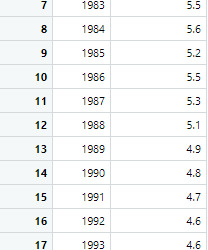
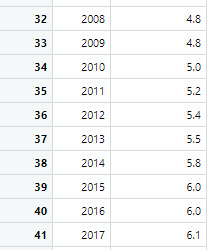
Dataset: This table shows the rates of male and females and the combined rates of both genders.

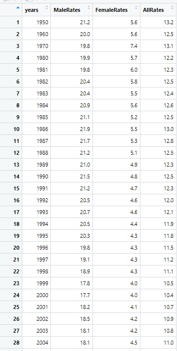
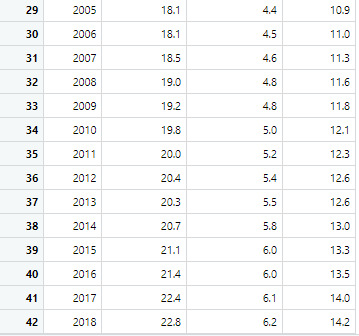
Source: https://catalog.data.gov/dataset/death-rates-for-suicide-by-sex-race-hispanic-origin-and-age-united-states-020c1

2. To start with my hypothesis, My hypothesis are:

H0: There is no difference between male and female suicide rates in the United States.

H1: There is a difference between male and female suicide rates in the United States.

3. Sample

The first sample is the male suicide rates and the second sample is the female suicide rates

4. Code in R Studio

MaleRates <- c(21.2, 20, 19.8, 19.9, 19.8, 20.4, 20.4, 20.9, 21.1, 21.9, 21.7, 21.2, 21, 21.5, 21.2, 20.5, 20.7, 20.5, 20.3, 19.8, 19.1, 18.9, 17.8, 17.7, 18.2, 18.5, 18.1, 18.1, 18.1, 18.1, 18.5, 19, 19.2, 19.8, 20, 20.4, 20.3, 20.7, 21.1, 21.4, 22.4, 22.8) FemaleRates <- c(5.6, 5.6, 7.4, 5.7, 6, 5.8, 5.5, 5.6, 5.2, 5.5, 5.3, 5.1, 4.9, 4.8, 4.7, 4.6, 4.6, 4.4, 4.3, 4.3, 4.3, 4.3, 4, 4, 4.1, 4.2, 4.2, 4.5, 4.4, 4.5, 4.6, 4.8, 4.8, 5, 5.2, 5.4, 5.5, 5.8, 6, 6, 6.1, 6.2) AllRates <- c(13.2, 12.5, 13.1, 12.2, 12.3, 12.5, 12.4, 12.6, 12.5, 13, 12.8, 12.5, 12.3, 12.5, 12.3, 12, 12.1, 11.9, 11.8, 11.5, 11.2, 11.1, 10.5, 10.4, 10.7, 10.9, 10.8, 11, 10.9, 11, 11.3, 11.6, 11.8, 12.1, 12.3, 12.6, 12.6, 13, 13.3, 13.5, 14, 14.2) years <- c(1950, 1960, 1970, 1980, 1981, 1982, 1983, 1984, 1985, 1986, 1987, 1988, 1989, 1990, 1991, 1992, 1993, 1994, 1995, 1996, 1997, 1998, 1999, 2000, 2001, 2002, 2003, 2004, 2005, 2006, 2007, 2008, 2009, 2010, 2011, 2012, 2013, 2014, 2015, 2016, 2017, 2018) Rates = data.frame(years, MaleRates, FemaleRates, AllRates) Rates1 = data.frame(years, MaleRates) Rates2 = data.frame(years, FemaleRates)

t.test(MaleRates, FemaleRates)

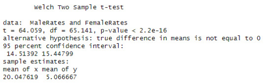
i. The sample means: MaleRates = 20.047619 and FemaleRates = 5.066667

ii. P-value = 0.00000000000000022

iii. Significance value of a = 0.05. P-value <= Significance level.

iv. 0.00000000000000022 <= 0.05. Since the p value is less than or equal to the significance level it indicates a significant difference between the two means.

This is the code for the line chart:

ggplot(data = Rates, aes(x = years, group = 2)) + geom_line(aes(y = MaleRates, color = "Male"), size = 1.2) + geom_line(aes(y = FemaleRates, color = "Female"), size = 1.2) + geom_line(aes(y = AllRates, color = "All"), size = 1.2) + labs(title = "Suicide Rates in the United States Over the Years", x = "Years", y = "Rates") + scale_color_manual(values = c("Male" = "blue", "Female" = "red", "All" = "green")) + theme_minimal()

5. Conclusion

There is a significant difference between the two sample means, and P-value <= Significance level, therefore I can conclude the the alterative hypothesis is true.

There is a significance difference in the male suicide rate and the female suicide rate in the United States.

[usfstatstudent]

Module 12 assignment

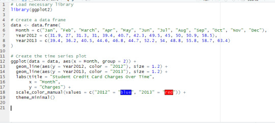
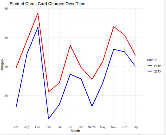
I used this model to compare the different years of 2012 and 2013 with the same variable of student credit card charges. The reason I used this type of chart was because it was better for comparing the two over time.

[usfstatstudent]

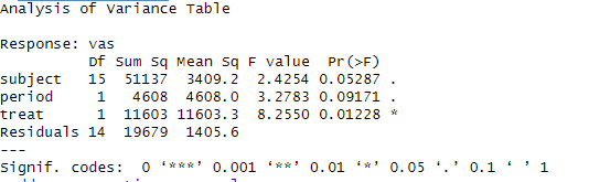
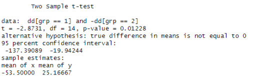
Module 11 Assignment

#Importing Data

library(ISwR)

ashina$subject <- factor(1:16)

attach(ashina)

act <- data.frame(vas=vas.active, subject, treat=1, period=grp)

plac <- data.frame(vas=vas.plac, subject, treat=0, period=ifelse(grp==1,2,1))

ashina.long <- rbind(act, plac) >

ashina.long$treat <- factor(ashina.long$treat)

ashina.long$period <- factor(ashina.long$period)

fit.ashina <- lm(vas ~ subject + period + treat, data = ashina.long) drop1(fit.ashina)

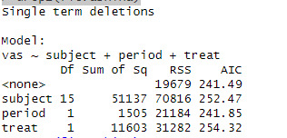
anova(fit.ashina)

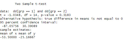
dd <- vas.active - vas.plac

t.test(dd[grp==1], -dd[grp==2],var.eq=T)

t.test(dd[grp==1], dd[grp==2], var.eq=T)

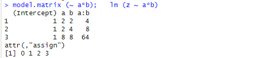
a <- g1(2, 2, 8) b <- g1(2, 4, 8) x <-- 1:8 y <- c(1:4, 8:5) z <- rnorm (8)

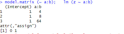
model.matrix(~ a:x); lm (z ~ a:x) model.matrix(~ ax); lm (z ~ aX) model.matrix(~b(x+y)); lm (z ~ b(x +y))

R will reduce the set of the design variables for an interaction term between the categorical variables when a main event is present but it will not detect the singularity caused by the interception. There is no singularities in the first two cases, however the last example has a coincidental singularity.

[usfstatstudent]

Module 10 Assignment

library(base) library(ISwR) cystfibr attach(cystfibr) linearmodel <- lm(pemax ~ age + weight + bmp + fev1, data = cystfibr) summary(linearmodel) anova(linearmodel) anovamodel <- aov(pemax ~ age + weight + bmp + fev1, data = cystfibr) summary(anovamodel)

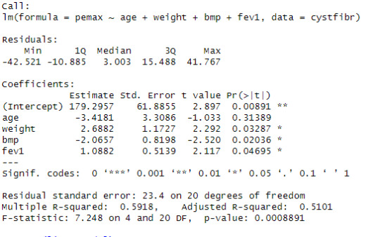
Looking at the linear progression model, we can see that the estimate of the value for the intercept is 179.2957 with significant p-value. The estimate of the variable age is -3.4181 for that unit change in the variable age in the dependent variable pemax with a non-significant p-value. The estimate of the variable weight is 2.6882 for that unit change in the variable weight in the dependent variable pemax with a significant p-value. The estimate of the variable bmp is -2.0657 for that unit change in the variable bmp in the dependent variable pemax with a significant p-value. The estimate of the variable fev1 is 1.0882 for that unit change in the variable fev1 in the dependent variable pemax with a significant p-value.

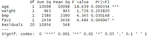
Looking at the ANOVA table, see that the p value of age is 0.00354, less than 0.001 so, we can reject the null hypothesis and can interpret it as the variation the effect of the variable age on the dependent variable pemex is not equal to zero. The p value of weight is 0.203820, greater than 0.05 so, we can not reject the null hypothesis and can interpret it as the variation the effect of the variable weight on the dependent variable pemex is equal to zero. The p value of bmp is 0.050148, less than or equal to 0.05 so, we can reject the null hypothesis and can interpret it as the variation the effect of the variable bmp on the dependent variable pemex is not equal to zero. The p value of fev1 is 0.046947, less than or equal to 0.05 so, we can reject the null hypothesis and can interpret it as the variation the effect of the variable fev1 on the dependent variable pemex is not equal to zero.

Importing Data

library(ISwR) Data <- secher head(Data)

Creating a model using birthweight and biparietal diameter

model1 <- lm(log(bwt) ~ log(bpd) , data = Data) summary(model1)

Creating a model using birthweight and abdominal diameter

model2 <- lm(log(bwt) ~ log(ad), data = Data) summary(model2)

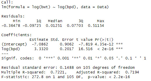
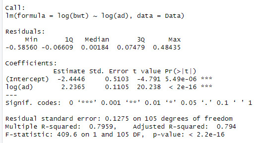
When looking at the data, we can see that the log(bpd) is a significant variable of the log(ad). The model also explains 79.5% of the variation in log(bwt)

Creating a model using birthweight and both abdominal and biparietal diameter

model3 <- lm(log(bwt) ~ log(ad) + log(bpd), data = Data) summary(model3)

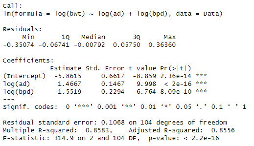
We can see that when both variables are added that the significance and Rsqaured increases to 85.5%.

The interpretation is, when there is a 1% increase in abdominal diameter increases the birthweight by 1.4667% and when there is a 1% increases in the biparietal diameter there is a 1.5519% increase in the birthweight.

[usfstatstudent]

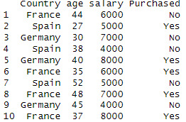
Module 9 Assignment

 assignment_data <- data.frame( Country = c("France","Spain","Germany","Spain","Germany", "France","Spain","France","Germany","France"), age = c(44,27,30,38,40,35,52,48,45,37), salary = c(6000,5000,7000,4000,8000), Purchased=c("No","Yes","No","No","Yes", "Yes","No","Yes","No","Yes"))

data <- assignment_data data

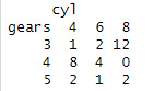
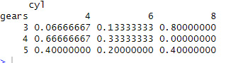
assignment9 <- table(mtcars$gear, mtcars$cyl, dnn =c("gears","cyl")) assignment9

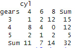
addmargins(assignment9)

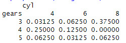
prop.table(assignment9)

prop.table(assignment9,margin = 1)

[usfstatstudent]

Module 8 Assignment

Report on drug and stress level by using R. Provide a full summary report on the result of ANOVA testing and what does it mean. More specifically, report  using the following R functions: Df, Sum, Sq Mean, Sq, F value, Pr(>F)

High_Stress <- c(10,9,8,9,10,8) Moderate_Stress <- c(8,10,6,7,8,8) Low_Stress <- c(4,6,6,4,2,2)

Stress_Data <- data.frame(StressLevel = c(High_Stress, Moderate_Stress, Low_Stress), Group = rep(c("High Stress", "Moderate Stress", "Low Stress"), each = 6)) ANOVA_Results <- aov(StressLevel ~ Group, data = Stress_Data)

summary(ANOVA_Results)

The Degrees of Freedom = 2, The total sum of the squares = 82.11, the mean of the square = 41.06, the F value = 21.36 and the P value = 4.08e-05.

install.packages("ISwR") library("ISwR")

data("zelazo") unlist(zelazo) active <-c(9.00,9.50,9.75,10.00,13.00,9.50) passive <-c(11.00, 10.00, 10.00,11.75,10.50,15.00) none <-c(11.50,12.00,9.00,11.50,13.25,13.00) ctr_8w1 <- c(13.25,11.50,12.00,13.50,11.50, 0) zelazo_data <- data.frame(ReactionTime= c(active,passive,none,ctr_8w1), group=rep(c("Active","Passive","None","Ctr.8w"),each=6))

AnoVA_Results = aov(ReactionTime ~ group, data = zelazo_data)

summary(AnoVA_Results)

Df = 3, Sum Sq = 11.08, Mean Sq = 3.694, F Value = 0.433, pr(>F) = 0.732

[usfstatstudent]

Module 7

1.1: x <- c(16, 17, 13, 18, 12, 14, 19, 11, 11, 10) y <- c(63, 81, 56, 91, 47, 57, 76, 72, 62, 48)

cor(x,y)

[1] 0.7282365. This value represents that there is a positive linear relationship between the predictor and the response variable.

1.2

Regression_model1=1m(y~x)

Regression_model$coefficients

intercepts = 19.205597 and 3.269107

2.1

The value of 0.9013 shows that there is a strong positive relationship

between the two varibles.

2.2

cov(x,y)/y^2 = 9.5349/141.1343 = 0.0676

(x-mean of x) = 0.0676y - 4.6081

x = 0.0676y - 4.6081 + 3.072

x = 0.0676y - 1.5361

a = -1.5361 b = 0.0676

2.3 If y = 80 minutes

x = - 1.5361 + 0.0676(80) = -1.5361 + 5.4080 = 3.8719

X approximately equals 3.9719

3.1

Examine the relationship Multi Regression Model as stated above and its Coefficients using 4 different variables from mtcars (mpg, disp, hp and wt). Report on the result and explanation what does the multi regression model and coefficients tells about the data?

Looking at the output that was given, it showed that hp and wt have a significant relationship while mpg and disp have no significant relationship because the p-value is greater that the level of significane of 0.05

4.

Using library(ISwR) and plot(metabolic.rate~body.weight,data=rmr), we can find that the predicted metabolic rate for a body weight of 70 kg is 1305.394

[usfstatstudent]

Module 6 Assignment

1a.The mean of the population of 8, 14, 16, 10 11 = 11.8

1b. Sample 1 n = 8, 10 Sample n = 14, 16

1c. The mean of sample 1 = 9 and the mean of sample 2 = 15

The sd of sample 1 = 1.41 and the sd of sample 2 = 1.41

1d.

X X=U (x-u)^2

8, 10 9 1.41

14, 16 15 1.41

8, 14, 16, 10,11 11.8 3.19

2a. The distribution is expected to be normal if both np and nq are greater 10 since p = 0.95 and q = 0.05

np = 100 x 0.95 = 95

nq = 100 x 0.05 = 5, since nq < 10 it is not a normal approximation distribution

2b. The smallest value n would have to be for a normal approximation distribution would have to be 200 cause nq = 200 x 0.05 = 10

3.

sample = rbinom(100,10,0.5) print(sample)

[1] 3 4 4 5 6 6 4 3 6 7 5 6 8 6 5 5 4 6 6 7 3 7 6 7 6 4 6 6 4 6 7 5 6 5 6 3 4 2 3 3 7 [42] 8 6 8 7 3 5 6 6 9 5 4 7 5 5 7 7 5 5 4 7 5 3 6 4 5 6 4 6 4 5 4 5 5 7 5 6 6 7 5 7 2 [83] 7 7 4 6 6 7 6 5 7 5 3 5 3 3 6 4 4 6

This program generates 100 values for the number of heads you would get if you tossed a coin 10 times in each simulation. The parameter is 0.5 because there is a 50% chance of getting heads in each flip.

[usfstatstudent]

Correlation Analysis Homework

After looking at the data and using the formula for correlation coefficient which is the sum of x minus the mean of x times the sum of y minus the mean of y dived by the number of observations times the sum of squares x times the sums of squares y. After calculating the values I came up with r = 528.3 / (6)(9.3986)(9.3692) = 0.9999

When looking at the formula for Pearson correlation coefficient as the covariance of x and y divided by the standard deviation of x times the standard deviation of y we get r = 528.3 / √((530)(526.688)) = 0.9999

[usfstatstudent]

Probability Theory

A1. The probability of event A is 1/3

A2. The probability of event B is 1/3

A3. p(a or b) = 1/3 + 1/3 - 10/90 = 2/3 - 1/9 = 6/9 - 1/9 = 5/9

A4. p(a or b) does not equal p(a) + p(b) because if you just add the probability it would be 2/3 but since we subtract the probability of both a and b the probability of a or b is 5/9

B.

The answer provided would be true because he takes the probability of A1 and the probability of B given A1 and then divides it by the probability B by taking the probability of B given A1 and probability of B given A2

C.

dbinom(0, size=10, prob=0.20)

[1] 0.1073742

[usfstatstudent]

x <- c(10,2,3,2,4,2,5)

y <- c(20,12,13,12,14,12,15)

mean(x) [1] 4

mean(y) [1] 14

median(x) [1] 3

median(y) [1] 13

summary(x) Min. 2.0 1st Qu. 2.0 Median 3.0 Mean 4.0 3rd Qu. 4.5 Max. 10.0

summary(y) Min. 12.0 1st Qu. 12.0 Median 13.0 Mean 14.0 3rd Qu. 14.5 Max. 20.0

var(x) [1] 8.333333

var(y) [1] 8.333333

sd(x) [1] 2.886751

sd(y) [1] 2.886751

When looking at these 2 sets of data, we notice that the mean median and mode if the second set is 10 higher than the ones of the first set. However when we compare the range and the interquartile range they are both 8 and 2.5 for each set. Also when we compare the variance and standard deviation, we can see that the values are the same for both sets.

[usfstatstudent]

Module 2 Assignment

assignment2<- c(6,18,14,22,27,17,22,20,22) myMean <- function(assignment2) { return(sum(assignment2)/length(assignment2))

}

myMean(assignment2)

[1] 18.66667

What this function does is it takes in the data from the vector assignment 2 and it adds up the numbers to get the sum of the vector then it divides it by the length of the vector and returning the mean of the vector.