#the life and times of kb byte
Text
A farewell to KB Byte
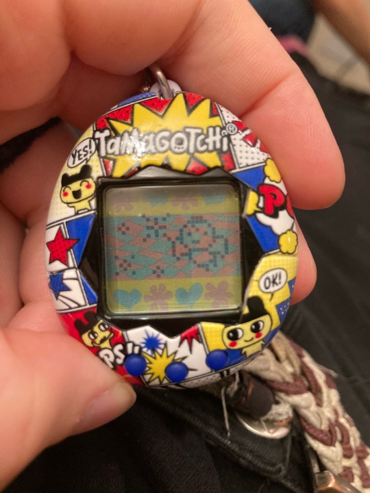
#the life and times of kb byte#tamagotchi#tamagotchi gen 1#tamagotchi p1#I realise that he probably would’ve died last night if I hadn’t paused him#day 8 (part 2)
6 notes
·
View notes
Note
According to the marvel comics, the entirety of Optimus Prime's personality and memories could be stored on a 5.25-inch Floppy disk. So I was wondering how much storage space is needed for the average Cybertronian mind?
Dear Megabyte Medium,
I thought I had answered this question recently, but now realize I only explained the part of the process which would be novel to a human. To recap: in the universe in question, through mass-shifting, we are able to represent around 400 VB of Cybertronian mental data on physical substrate which normally would accommodate 640 TB of data (and like humans, most of the time we require only 10% of our mental capacity at any given moment, which is mass-shifted up into RAM). The rest of the downsizing is simple data compression, just as you would use!
Though we are a long-lived race, the highly repetitive nature of our experiences and language allows for extremely efficient lossy compression. Millions of years of life on Cybertron may be expressed in just a few hundred bytes, our most complex philosophies may be expressed in one or two common dictionary strings—such as "better to fight and die", or "it never ends". The oldest and most developed Cybertronians have complex and nuanced personality subroutines, logical reasoning algorithms and long-term memory, in addition to the unique speech engrams and transformation schemas I previously mentioned, which can all be represented in less than 720 KB. Zachary was thus able to store Optimus Prime's entire mind on a 5 1/4 inch floppy disk and I believe he had enough space left over for a copy of Zork too.
#ask vector prime#transformers#maccadam#marvel transformers#optimus prime#cybertronian language#zork#complete-idiot-inc
12 notes
·
View notes
Photo
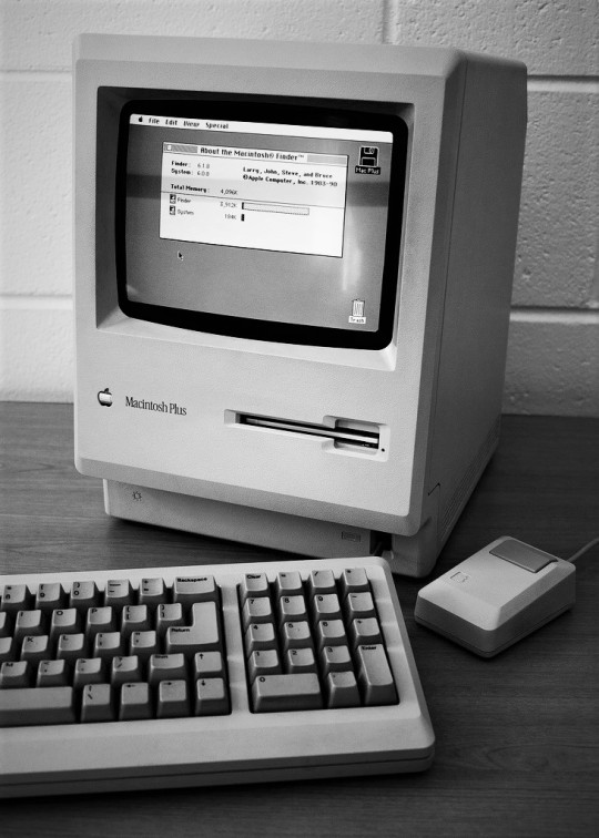
The Macintosh Plus computer is the third model in the Macintosh line, introduced on January 16, 1986, two years after the original Macintosh and a little more than a year after the Macintosh 512K, with a price tag of US$2599. As an evolutionary improvement over the 512K, it shipped with 1 MB of RAM standard, expandable to 4 MB, and an external SCSI peripheral bus, among smaller improvements. It originally had the same generally beige-colored case as the original Macintosh ("Pantone 453"), however in 1987, the case color was changed to the long-lived, warm gray "Platinum" color. It is the earliest Macintosh model able to run System 7 OS.
Bruce Webster of BYTE reported a rumor in December 1985: "Supposedly, Apple will be releasing a Big Mac by the time this column sees print: said Mac will reportedly come with 1 megabyte of RAM ... the new 128K-byte ROM ... and a double-sided (800K bytes) disk drive, all in the standard Mac box". Introduced as the Macintosh Plus, it was the first Macintosh model to include a SCSI port, which launched the popularity of external SCSI devices for Macs, including hard disks, tape drives, CD-ROM drives, printers, Zip Drives, and even monitors. The SCSI implementation of the Plus was engineered shortly before the initial SCSI spec was finalized and, as such, is not 100% SCSI-compliant. SCSI ports remained standard equipment for all Macs until the introduction of the iMac in 1998, which replaced most of Apple's "legacy ports" with USB.
The Macintosh Plus was the last classic Mac to have a phone cord-like port on the front of the unit for the keyboard, as well as the DE-9 connector for the mouse; models released after the Macintosh Plus would use ADB ports.
The Mac Plus was the first Apple computer to utilize user-upgradable SIMM memory modules instead of single DIP DRAM chips. Four SIMM slots were provided and the computer shipped with four 256K SIMMs, for 1MB total RAM. By replacing them with 1MB SIMMs, it was possible to have 4MB of RAM. (Although 30-pin SIMMs could support up to 16MB total RAM, the Mac Plus motherboard had only 22 address lines connected, for a 4MB maximum.)
It has what was then a new 3 1⁄2-inch double-sided 800 KB floppy drive, offering double the capacity of floppy disks from previous Macs, along with backward compatibility. The then-new drive is controlled by the same IWM chip as in previous models, implementing variable speed GCR. The drive was still completely incompatible with PC drives. The 800 KB drive has two read/write heads, enabling it to simultaneously use both sides of the floppy disk and thereby double storage capacity. Like the 400 KB drive before it, a companion Macintosh 800K External Drive was an available option. However, with the increased disk storage capacity combined with 2-4x the available RAM, the external drive was less of a necessity than it had been with the 128K and 512K.
The Mac Plus has 128 KB of ROM on the motherboard, which is double the amount of ROM in previous Macs; the ROMs included software to support SCSI, the then-new 800 KB floppy drive, and the Hierarchical File System (HFS), which uses a true directory structure on disks (as opposed to the earlier MFS, Macintosh File System in which all files were stored in a single directory, with one level of pseudo-folders overlaid on them). For programmers, the fourth Inside Macintosh volume details how to use HFS and the rest of the Mac Plus's new system software. The Plus still did not include provision for an internal hard drive and it would be over nine months before Apple would offer a SCSI drive replacement for the slow Hard Disk 20. It would be well over a year before Apple would offer the first internal hard disk drive in any Macintosh.
A compact Mac, the Plus has a 9-inch (23 cm) 512 × 342 pixel monochrome display with a resolution of 72 PPI, identical to that of previous Macintosh models. Unlike earlier Macs, the Mac Plus's keyboard includes a numeric keypad and directional arrow keys and, as with previous Macs, it has a one-button mouse and no fan, making it extremely quiet in operation. The lack of a cooling fan in the Mac Plus led to frequent problems with overheating and hardware malfunctions.
The applications MacPaint and MacWrite were bundled with the Mac Plus. After August 1987, HyperCard and MultiFinder were also bundled. Third-party software applications available included MacDraw, Microsoft Word, Excel, and PowerPoint, as well as Aldus PageMaker. Microsoft Excel and PowerPoint (originally by Forethought) were actually developed and released first for the Macintosh, and similarly Microsoft Word 1 for Macintosh was the first time a GUI version of that software was introduced on any personal computer platform. For a time, the exclusive availability of Excel and PageMaker on the Macintosh were noticeable drivers of sales for the platform.
The case design is essentially identical to the original Macintosh. It debuted in beige and was labeled Macintosh Plus on the front, but Macintosh Plus 1 MB on the back, to denote the 1 MB RAM configuration with which it shipped. In January 1987 it transitioned to Apple's long-lived platinum-gray color with the rest of the Apple product line, and the keyboard's keycaps changed from brown to gray. In January 1988, with reduced RAM prices, Apple began shipping 2- and 4- MB configurations and rebranded it simply as "Macintosh Plus." Among other design changes, it included the same trademarked inlaid Apple logo and recessed port icons as the Apple IIc and IIGS before it, but it essentially retained the original design.
An upgrade kit was offered for the earlier Macintosh 128K and Macintosh 512K/enhanced, which includes a new motherboard, floppy disk drive and rear case. The owner retained the front case, monitor and analog board. Because of this, there is no "Macintosh Plus" on the front of upgraded units, and the Apple logo is recessed and in the bottom left hand corner of the front case. However, the label on the back of the case reads "Macintosh Plus 1MB". The new extended Plus keyboard could also be purchased. Unfortunately, this upgrade cost almost as much as a new machine.
The Mac Plus itself can be upgraded further with the use of third-party accelerators. When these are clipped or soldered onto the 68000 processor, a 32 MHz 68030 processor can be used, and up to 16 MB RAM. This allows it to run Mac OS 7.6.1.
There is a program available called Mini vMac that can emulate a Mac Plus on a variety of platforms, including Unix, Windows, DOS, classic Mac OS, macOS, Pocket PC, iOS and even Nintendo DS.
Although the Macintosh Plus would become overshadowed by two new Macintoshes, the Macintosh SE and the Macintosh II in March 1987, it remained in production as a cheaper alternative until the introduction of the Macintosh Classic on October 15, 1990. This made the Macintosh Plus the longest-produced Macintosh ever, having been on sale unchanged for 1,734 days, until the 2nd generation Mac Pro, introduced on December 19, 2013, surpassed the record on September 18, 2018. (it would ultimately last for 2,182 days before being discontinued on December 10, 2019) It continued to be supported by versions of the classic Mac OS up to version 7.5.5, released in 1996. Additionally, during its period of general market relevance, it was heavily discounted like the 512K/512Ke before it and offered to the educational market badged as the "Macintosh Plus ED". Due to its popularity, long life and its introduction of many features that would become mainstays of the Macintosh platform for years, the Plus was a common "base model" for many software and hardware products.
Daily inspiration. Discover more photos at http://justforbooks.tumblr.com
17 notes
·
View notes
Text
Mel B and HAIM Color Bars Solve
In this post:
https://pangenttechnologies.tumblr.com/post/184051996657/melanie-brown-interviewed-by-piers-morgan-for
There are color bars across the bottom.
They don’t appear to be standard Pangent color codes
A very similar-looking set of color bars appeared in this HAIM post:
https://pangenttechnologies.tumblr.com/post/182280291497/support-six-incredible-causes-and-sit-vip-with
I think I got something valid for the second Haim image

it’s VERY green but i think those are all valid pangent colors
I just inverted the colors
Here is the first Haim image’s colors, this is just inverted from the original. It loooks valid to me

Here’s the Mel B “rumor comes out” colors, inverted. I think I was just really overthinking this, as just inverting the colors gives me something very green but valid (I think) in Pangent colors

here are the colors from inverting the “is Mel Brown gay” and “Haim sisters with Emma Stone” posts.
44 45 4c 49 53 57 4e 56 46 41 55 4c 4a 56 5a 4a 53 45 42 47 4c 50 53 55 4e
43 46 4e 54 4f 4a 41 56 4c 53 44 43 53 4d 4b 54 42 4b 4e 43 49 54 4f 47 54
DELISWNVFAULJVZJSEBGLPSUNCFNTOJAVLSDCSMKTBKNCITOGT
vig argentina:
DNFEFDFIFADFFIGBFEBPFLFBFPFNCIFNCDFDCBGGGICACICICG
A1Pf:
4d65646961466972652f6b626f6d396d346432777931393937
hex:
MediaFire/kbom9m4d2wy1997
http://mediafire.com/?kbom9m4d2wy1997
KansasCity1997.zip -> argentina_ascii.wav
It’s a Kansas City Standard (KCS) Wav File
decode to text using Python and these scripts:
http://www.dabeaz.com/py-kcs/
It starts off with a code:
khg tey begww nfmkuk mrcm
deykipn qp ko evqp nivo ltd
i'xl qlue of qted ww rzn
i'o mmrytkuk mrcm
pj sv ttpid ko uoye de fvay rgcpr
t'cl uoye yio kshe
vigenere rachel:
the man keeps coming back
wanting me to come with him
i’ve made my mind up now
i’m fighting back
if he tries to shut me down again
i’ll shut him down
The rest is an ASCII photo of Lottie/Argentina.


Second image:
Lime Black Cyan Blue Cyan Orange Cyan Yellow Cyan Yellow Lime Lime Lime Green Lime Green Cyan Red Lime Green Cyan White Cyan Lime Cyan Yellow Lime Green Lime Brown Lime Orange Cyan Red Lime Grey Dark-Grey Lime Lime Cyan Yellow Lime Grey Lime Green Lime Pink Cyan Red
Cyan Lime Lime Black Cyan Orange Cyan Lime Lime Blue Lime Green Lime Green Cyan Red Cyan Yellow Cyan Orange Cyan Cyan Cyan Lime Lime Orange Lime Green Lime Blue Lime Dark-Grey Cyan Orange Lime Black Lime Black Cyan Lime Lime Not-so-Brown Lime Brown Lime Blue black black black black
4F 56 52 53 53 44 49 49 51 49 5 05 4 5 3 4 9 4 A 4 2 5 1 4 D 4 E 4 4 5 3 4 D 4 9 4 7 5 1
5 4 4 F 5 2 5 4 4 6 4 9 4 9 5 1 5 3 5 2 5 5 5 4 4 2 4 9 4 6 4 E 5 2 4 F 4 F 5 4 4 B 4 A 4 6 X X X X
OVRSSDIIQIPTSIJBQMNDSMIGQ
TORTFIIQSRUTBIFNROOTKJF
decodes with vig password limonada to:
DNFEFDFIFADFFIGBFEBPFMFGF
LCDGFFIFKFGGBFFCJCAGKGF
decodes to
4 d 6 5 6 4 6 9 6 1 4 6 6 9 7 2 6 5 2 f 6 c 6 7 6
b 3 4 7 6 6 9 6 a 6 7 7 2 6 6 3 0 3 1 7 a 7 6
MediaFire/lgk4vijgrf01zv
http://mediafire.com/?lgk4vijgrf01zv
which isnt valid
Remember the missing bytes at the end?
yeah i’m just trying any numbers and letters
i think we’re missing a letter or two
http://www.mediafire.com/?lgk4vijgrf01zvc
KansasCity1996.zip -> limonada_ascii.wav
Audio in Kansas City Standard (KCS) format. Outputs text including ASCII art and vigenered text

k rbf'v eohl ai tuel vyc
spm $gtm hbsu c mlewoxj $cjr
twb ky'jl mfupc wh l uaqyw cvr cl’$ i$ll yccyy vc twv eclkl
c poa'l yh$o jcj dqvu c uhh werh ritfi huau
$svgvn, olrsb cykvoydcbwif
oufe $qgywx kb g$g uclfphs
nbl hbll ocefkvu ynll oo$wg
bllg alkgtt $gy nte ewgn $x vw$w
yponwcyd tves qp $cjr $g$s
m$l’m etemuawapu nycqbml pn, yoew oho eqfr
spl hbwyy'e lrkg uyv nsfk qn vyj
tukbr a’$f umuh ywv psl tl
qtornsl d$g wf fqe
qbgvmq tb khia ewfqwtqba $ll
wnbowhr ljog a hiwfwk wamcdsnpda
yagyqba louf i'iw ycwdgr rng$mn$phs i ygjyo sdchl jmf
w$vieiay hi waxs javp as xhcxuew
ticwxse
ap lsulo ue i qar cy dktr
lq uoew muulhjs gj xtwrff
a vigenere solver says the key is “conscioushumansouls” but it seems to have decoded with errors
the dollar signs being errors here
changing them to Z gives me this
“”“**
i don’t want to hurt her
any more than i already have
but we’re stuck in a cycle and it’s only going to get worse
i don’t know how long i can keep doing this
reboot, clean installation
hate myself in the morning
not that morning ever comes
hate myself for the rest of time
whatever time we have here
she’s struggling against it, more and more
and there’s less and less of her
maybe i’ll just let her be
whoever she is now
choose to stop murdering her
knowing that i failed completely
knowing that i’ve killed everything i loved about her
choosing to live with my failure
forever
in death as i did in life
to make failure my friend
”“”**
this text later appeared in video “mountain”
https://vimeo.com/410088899
For this Mel B inverted mostly green border image, I’ve got my first swing at a transcription: https://i.imgur.com/JmSqveN.jpg
46 44 4f 45 4c 4e 47 4f 49 45 4f 4f 49 53 49 52 46 49 49 52 55 52 47 41 4d 47 49
44 49 52 4c 46 4f 45 54 49 4f 4e 46 4e 52 4e 52 48 41 52 52 52 47 52 55 47 4d 49
FDOELNGOIEOOISIRFIIRURGAMGI
DIRLFOETIONFNRNRHARRRGRUGMI
might be (should be?) vigenere but obvious choices didnt work. backwards maybe??
oh that’s weird
IMGURGRRRAHRNRNFNOITEOFLRID
IGMAGRURIIFRISIOOEIOGNLEODF
backwards it says imgur.
maybe a coincidence, but maybe it’s already a reduced alphabet ??
letters included in string are:
adefghilmnorstu
eh i guess not
IGMAGRURIIFRISIOOEIOGNLEODF
IMGURGRRRAHRNRNFNOITEOFLRID
and with IMGUR removed I noticed it had GARFIELD too… I later saw that all this has been done before for another solve…
IGMAGRURIIFRISIOOEIOGNLEODF
77 6 8744 74E5 14 A
I M G URII R SIOO IOGN EO F
G A R F I E L D
IMGURGRRRAHRNRNFNOITEOFLRID
666 9 565 54 2 4A 67
IMGUR RRR H NRN NO T OF RI
G A R F I E L D
gives
https://i.imgur.com/whtGNQJ.jpg
and
https://i.imgur.com/fiVUBJg.jpg
First is “removed”, so I don’t know if that was the expected solution or if I made a mistake or if it’s been removed from imgur because we took too long.
Other one is correct though. - Geri Halliwell’s Elvis Costume

1 note
·
View note
Text
Beginner Problems With TCP & The socket Module in Python
This is important information for beginners, and it came up in Discord three times already, so I thought I’d write it up here.
The Python socket module is a low-level API to your operating system’s networking functionality. If you create a socket with socket.socket(socket.AF_INET, socket.SOCK_STREAM), it does not give you anything beyond ordinary TCP/IP.
TCP is a stream protocol. It guarantees that the stream of bytes you send arrives in order. Every byte you send either arrives eventually, unless the connection is lost. But if a TCP packet of data goes missing, it is sent again, and if TCP packets arrive out of order, the data stream is assembled in the right order on the other side. That’s it.
If you send data over TCP, it may get fragmented into multiple packets. The data that arrives is re-assembled by the TCP/IP stack of the operating system on the other side. That means that, if you send multiple short strings through a TCP socket, they may arrive at once, and the reader gets one long string. TCP does not have a concept of “messages”. If you want to send a sequence of messages over TCP, you need to separate them, for example through a line break at the end of messages, or by using netstrings. More on that later in this post!
If you don’t do that, then using sockets in Python with the socket module will be painful. Your operating system will deceive you and re-assemble the string you sock.recv(n) differently from the ones you sock.send(data). But here is the deceptive part. It will work sometimes, but not always. These bugs will be difficult to chase. If you have two programs communicating over TCP via the loopback device in your operating system (the virtual network device with IP 127.0.0.1), then the data does not leave your RAM, and packets are never fragmented to fit into the maximum size of an Ethernet frame or 802.11 WLAN transmission. The data arrives immediately because it’s already there, and the other side gets to read via sock.recv(n) exactly the bytestring you sent over sock.send(data). If you connect to localhost via IPv6, the maximum packet size is 64 kB, and all the packets are already there to be reassembled into a bytestream immediately! But when you try to run the same code over the real Internet, with lag and packet loss, or when you are unlucky with the multitasking/scheduling of your OS, you will either get more data than you expected, leftover data from the last sock.send(data), or incomplete data.
Example
This is a simplified, scaled-down example. We assume that data is sent in packets of 10 bytes over a slow connection (in real life it would be around 1.5 kilobytes, but that would be unreadable). Alice is using sock.sendall(data) to send messages to Bob. Bob is using sock.recv(1024) to receive the data. Bob knows that messages are never longer than 20 characters, so he figures 1024 should be enough.
Alice sends: "(FOO)"
Bob receives: "(FOO)"
Seems to work. They disconnect and connect again.
Alice sends: "(MSG BAR BAZ)"
Bob receives: "(MSG BAR B" - parsing error: unmatched paren
How did that happen? The maximum packet size supported by the routers of the connection (called path MTU) between Alice and Bob is just 10 bytes, and the transmission speed is slow. So one TCP/IP packet with the first ten bytes arrived first, and socket.recv(1024) does not wait until at least 1024 bytes arrive. It returns with any data that is currently available, but at most 1024 bytes. You don’t want to accidentally fill all your RAM!
But this error is now unrecoverable.
Alice sends: "(SECOND MESSAGE)"
Bob receives: "AR)(SECOND ME" - parsing error: expected opening paren
The rest of the first message arrived in the mean time, plus another TCP packet with the first part of another message.
Alice and Bob stop their programs and connect again. Their bandwidth and path MTU are now higher.
Alice sends: "(FOOBAR)"
This time Bob’s PC lags behind. The Java update popup hogs all the resources for a second.
Alice sends: "(SECOND MESSAGE)"
Bob receives "(FOOBAR)(SECOND MESSAGE)" - parsing error: extra data after end of message
If Bob had tried to only read 20 bytes with sock.recv(20) - because a message can never be longer than 20 bytes - he would have gotten "(FOOBAR)(SECOND MESS”.
And the same code would have run without a hitch when connected to localhost!
Additionally, the sock.send(data) method might not send all the data you give to it! Why is that? Because maybe you are sending a lot of data, or using a slow connection, and in that case send() just returns how much of the data you gave it could be sent, so your program can wait until the current data in the buffer has been sent over the network. This is also a kind of bug that is hard to track down if you’re only connecting to localhost over the loopback device, because there you have theoretically infinite bandwidth, limited only by the allocated memory of your OS and the maximum size of an IP packet. If you want all your data to be sent at once, guaranteed, you need to use sock.sendall(data), but sendall will block, that means your program will be unresponsive until all the data has been sent. If you are writing a game, using sendall on the main thread will make your game lag - this might not be what you want.
Solutions
You can use socketfile=socket.makefile() and use socketfile.readline() on that object. This is similar to java.io.BufferedReader in java: f.readline() gives you one line, it blocks until all the data until the next linebreak is received, and it saves additional data for the next call to readline. Of course, you also have to delimit the data you send by appending "\n" at the end of your message.
You can also use netstrings. Netstrings encode data by prepending the length of the incoming data to a message. The pynetstring module with the pynetstring.Decoder wrapper gives you a simple interface similar to readline.
If you want to send individual short messages, and don’t care if some of them get lost, you might want to look into UDP. This way, two messages will never get concatenated. Why would you want to send individual packets that might get lost? Imagine a multiplayer game where your client sends the current position of the player to the server every frame, delimited by commas and linefeeds like this “123.5,-312\n“. If a TCP packet gets lost, it is re-sent, but by that time, the player is already somewhere else! The server has to wait until it can re-assemble the stream in the right order. And the server will only get the latest position from the client after the earlier position, which is now outdated, has been re-sent. This introduces a lot of lag. If you have 5% packet loss, but you send a UDP packet with the player position every frame, you can just add time current frame number to the message, e.g. “5037,123.5,-312\n“ if that message gets lost or takes along time to deliver, and the next message is “5038,123.5,-311.9\n“, the server just updates to the newest coordinates. If a package with a timestamp older than the newest known timestamp arrives, it is ignored.
Lastly, you could do a request-response protocol, where the server responds with “OK\n“ or something like that whenever it has processed a message, and the client waits to send additional data until an OK is received. This might introduce unacceptable round-trip lag in real-time games, but is fine in most other applications. It will make bi-directional communication more difficult, because you cannot send messages both ways, otherwise both sides can send a message at the same time, expect to get an OK response, but receive something that is not an OK response instead.
Further Reading
https://en.wikipedia.org/wiki/Path_MTU_Discovery
https://en.wikipedia.org/wiki/IP_fragmentation
http://cr.yp.to/proto/netstrings.txt
https://pypi.org/project/pynetstring/
3 notes
·
View notes
Text
Six Step Guidelines for Health

We then design an inference engine that combines the health metric alerts. Remembers when the Gallup World Poll was first conceived in 2005. He says that the survey design workforce consulted with some prime minds - together with the Nobel Prize-winners Daniel Kahneman, psychologist, and economist Angus Deaton - and determined to incorporate two different types of happiness questions in the poll: one that is an general "life analysis" from zero to 10, and one other that focuses on the emotional experiences of each day life. In swedish massage , we first describe the involved mental health dimensions and introduce the motivation of our assessment strategy. The first one is BM25 Robertson and Zaragoza (2009) and the other one relies on a site-particular Sentence-BERT (SBERT) Reimers and Gurevych (2019). Because of the limited sources, we indexed the various search engines with the subset of the TREC corpus. A technique is to consider surrounding phrases of the disease words that may give the context of the text. In abstract, the pattern dimension and the number of observations per particular person of the processed AURORA information will provide reasonable parameter estimation and BIC-based mannequin selection results.

youtube
The exploitation of this by attackers (e.g., as a reflector) will manifest in an alert when the NELF metric becomes excessive, whereas LEF is also high (in case the queries are malformed or non-existent). 5 × drop of vitality consumption for the latter case is as a result of low traffic load transmitted to the cloud. Three × more vitality efficient, the degradation by way of accuracy compared to greater ones is just too essential. This work proposes an environment friendly injury detection resolution at the edge, concurrently lowering community visitors and energy consumption, while anomaly detection accuracy will not be adversely altered in comparison with cloud-based techniques. Additionally, we exhibit the embedding of our tuned pipeline on a tiny low power gadget, moving the harm detection to the sting of the network. Furthermore, we offer a quick evaluation of the outcomes by utilizing the ability of explainable AI. Notice that we ship one hour of acquired information all at the identical time to leave NB-IoT in the facility sleep mode (PSM) for most of the time, lowering the full power consumption. NB-IoT deployment of nationally-licensed connectivity (e.g., LTE bands) implies no band usage limitation and no latency for streaming acquired data to the cloud.
It exhibits that exploiting the full deployment of the cloud computing method consumes 312.848 J/h the place it reduces to 63.508 J/h for the localized sensor deployment of our pipeline. Tab. IV stories the deployment results of model inference on the node. Each node within the graph signifies a doc from the examined dataset that has been mentioned by one other doc. Also, we used quality estimators based on RoBERTa models trained on the Health News Review dataset as a reranking model. Thanks to this efficiency, we imagine DescEmb can open new doors for big-scale predictive models when it comes to operational price in finance and time. 5.Eight % over the state-of-the-art when it comes to F1 score. One of the best answer in terms of accuracy, i.e., the PCA with 5 seconds input window dimension, consumes 73.96 uJ. POSTSUPERSCRIPT ×, from 780 KBytes/hour to 10 Bytes/hour, in comparison with a cloud-based mostly anomaly detection resolution. Transition prices to develop a scalable resolution for SHM functions. Forty eight %, on our SHM dataset collected on a real-standing Italian bridge. ∼ 780 kB/hour) for a complete cloud-based mostly strategy prohibits its utilization for giant-scale SHM eventualities.
The cloud-primarily based methodology constantly streamlines the data to the cloud for each the coaching and detection phases. The task of early detection is driven by social engagements of the information article captured within a fixed time frame. First, we propose a new injury detection pipeline, comprising a pre-processing step, an anomaly detection algorithm, and a postprocessing step. Let us illustrate the positioning with an instance. For instance a tweet “I made such an excellent bowl of soup I think I cured my very own depression” contains a illness of “depression” however this is used figuratively. The enter textual content is gathered from the social media platforms akin to Twitter, Facebook, Reddit, etc. The gathering process includes crawling the aforementioned platforms based on keywords containing disease names. The keyword-based mostly information collection doesn't consider the context of the text and therefore contains irrelevant data. Utilize emojis within the text to assist enhance the classification outcomes. Figurative and non-health mention of disease words makes the classification process difficult. Non-health and a figurative mention of illness words in these instances pose challenges to the HMC.
Health mentioning classification (HMC) classifies an input text as health mention or not. Health mentioning classification (HMC) offers with the classification of a given piece of a textual content as health point out or not. In this manner, it achieves the contextual representation of a given word. Additionally, we utilize contrastive loss that pushes a pair of clean and perturbed examples shut to each other and different examples away in the illustration area. We generate adversarial examples by perturbing the embeddings of the model and then practice the model on a pair of fresh and adversarial examples. The important thing thought is so as to add a gradient-primarily based perturbation to the enter examples, after which practice the mannequin on each clear and perturbed examples. AdaEM depends on two key ideas. The schema for person and content data are comparable and embody metrics, key efficiency indicators (KPIs) and traits. Θ are learnable modeling parameters. With this in thoughts, energy consumption is the one counter impact of larger input dimensions, whereas different elements like memory footprint and execution time are happy. We wish to quantify each of those situations regarding vitality consumption. In our paper herein, we present a peculiar Multi-Task Learning framework that jointly predicts the impact of SARS-CoV-2 as well as Personal-Protective-Equipment consumption in Community Health Centres with respect to a given socially interacting populace.

For the number of cohorts, start year, gender, and area have been chosen as partitioning standards in this paper in an effort to observe the returns of education to health fairness in cohorts with generational, gender, and regional differences. Out of 100 points, the Tree Equity Score considers existing tree canopy, inhabitants density, earnings, employment, floor temperature, race, age and health. The node put in on the viaduct works with an output sampling rate of a hundred Hz; thus, it generates a hundred 16-bits samples per second. We apply our technique to identify over one hundred completely different DNS belongings throughout the two organizations, and validate our results by cross-checking with IT staff. However, contextual representations have improved the performance of the classifier over non-contextual representations. To deal with the issue of data sparsity and help the automation of the 3-Step principle over social media knowledge Klonsky and will (2015), the info augmentation over psychological healthcare may give exceptional results. The key problem on this domain is to avail the ethical clearance for utilizing the person-generated text on social media platforms.
0 notes
Text
The Invention of Computers - Secrets of the 1970s - Ulzzang Korea
The Invention of Computers Secrets of the 1970s:
Hello,
I'm Emon. I'm using my own knowledge and research The invention of computers secrets of the 1970s
The 1970s were a heady time in the computer industry. The decade saw many notable inventions and developments, especially in the areas of the personal computer, networking, and object-oriented programming. Innovators produced groundbreaking hardware and software. Several large organizations entered the industry or expanded during the decade, including Texas Instruments, Xerox and International Business Machines, or IBM. Some companies, such as RCA, dipped their toes in industry waters, but quickly withdrew from the computer scene.

Major computer events in 1970:
IBM introduced the System/370 that included the use of Virtual Memory and utilized memory chips instead of magnetic core technology.
Intel introduces the first ALU (arithmetic logic unit), the Intel 74181.
Other computer events in 1970
The Unix time, aka epoch time, was set to start on January 1, 1970.
China's first satellite, the "Dong Fang Hong I," was launched into space on April 24, 1970.
The Luna 16 probe returned on September 24, 1970, and became the first unmanned Moon mission to return lunar samples.
The first commercially available RAM chip was the Intel 1103, which was released in October 1970.
Douglas Engelbart's patent (3,541,541) was granted for the first computer mouse on November 17, 1970.
E. F. Codd at IBM formally introduced relational algebra.
The International Standard for Organization made the ten-digit ISBN official.
Steve Crocker and the UCLA team released NCP.
The Sealed Lead Acid battery began its commercial use.
The Bloom filter data structure was first proposed by scientist Burton Howard Bloom at MIT in 1970.
Jack Kilby was awarded the National Medal of Science.
New computer products and services introduced in 1970:
Intel released its first commercially available DRAM, the Intel 1103 in October 1970. Capable of storing 1024 bytes or 1 KB of memory.
Intel announced 1103, a new DRAM memory chip containing more than 1,000 bits of information. This chip was classified as random-access memory (RAM).
The Forth programming language was created by Charles H. Moore.
U.S. Department of Defense developed ADA, a computer programming language capable of designing missile guidance systems.
Philips introduced the VCR in 1970.
John Conway released Game of Life.
Computer companies founded in 1970
Henry Edward Roberts established Micro Instrumentation and Telemetry Systems (MITS) in 1970.
Waytek was founded in 1970.
Western Digital was founded in 1970.
The Xerox Palo Alto Research Center (PARC) was established in 1970 to perform basic computing and electronic research.
The International typeface Corp. (ITC) was founded in 1970.
0 notes
Text
Black Panther 2018 Bluray Download

The game features high-impact two vs. It is the third Dragon Ball Z game for the PlayStation Portable, and the fourth and final Dragon Ball series game to appear on said system. It has a score of 63% on Metacritic. GameSpot awarded it a score of 6.0 out of 10, saying “Dragon Ball Z: Tenkaichi Tag Team is just another DBZ fighting game, and makes little effort to distinguish. Dbz tenkaichi tag team mods. Dragon Ball Z Tenkaichi Tag Team Mod (OB3) is a mod game and this file is tested and really works. Now you can play it on your android phone or iOS Device. Game Info: Game Title: Dragon Ball Z Tenkaichi Tag Team Mod Best Emulator: PPSSPP Genre: Fighting File Size: 617 MB Image Format: CSO. The Ultimate tenkaichi tag team fight 2 with different battle universe: son the goku super ultra instinct battle saiyan world, the Xeno verse's 2 fighting dragon tournament ball world super Z Saiyan 4 Blue, vegeta wit kakarot super dragon ultra saiyan instinct in the universe tournament of the power ball stay 1 vs 1 son with gohan magic goku super Z battle saiyan.
Pirivom santhipom songs free download. Black Panther is a 2018 superhero and action Hollywood movie are based on marvels comics, whereas Chadwick Boseman has played the lead role in this movie. The movie was released on 29 January 2018 and this 2018 Superhit Hollywood movie. Below in this article, you can find the details about Black Panther Full Movie Download and where to Watch Black Panther. Black panther 2018 720p bluray x264 yts am Subtitles Download. Download Black panther 2018 720p bluray x264 yts am Subtitles (subs - srt files) in all available video formats. Subtitles for Black panther 2018 720p bluray x264 yts am found in search results bellow can have various languages and frame rate result. For more precise subtitle search.
Black Panther 2018 online, free
Download Hollywood Movies 2018 Black Panther
Black Panther 2018 Film
Black Panther 2018 Download Free
Black Panther (2018)
Action / Adventure / SciFi
Chadwick Boseman, Michael B. Jordan, Lupita Nyong o, Danai Gurira, Martin Freeman, Daniel Kaluuya, Letitia Wright, Winston Duke, Sterling K. Brown, Angela Bassett, Forest Whitaker, Andy Serkis, Florence Kasumba, John Kani, David S. Lee
T Challa, heir to the hidden but advanced kingdom of Wakanda, must step forward to lead his people into a new future and must confront a challenger from his country s past.
File: Black.Panther.2018.720p.BluRay.H264.AAC-RARBG.mp4
Size: 1746594277 bytes (1.63 GiB), duration: 02:14:33, avg.bitrate: 1731 kb/s
Audio: aac, 48000 Hz, 5:1 (eng)
Video: h264, yuv420p, 1280x536, 23.98 fps(r) (und)
RELATED MOVIES
#195stars
Chris Hemsworth, Tom Hiddleston, Cate Blanchett, Mark Ruffalo
plot
Imprisoned on the planet Sakaar, Thor must race against time to return to Asgard and stop Ragnarok, the destruction of his world, at the hands of the
Action / Adventure / Comedy / Fantasy / SciFiBRRIP#667stars
Chris Evans, Robert Downey Jr., Scarlett Johansson, Sebastian Stan
plot
Political involvement in the Avengers affairs causes a rift between Captain America and Iron Man.
Action / Adventure / SciFiBRRIP#429stars
Benedict Cumberbatch, Chiwetel Ejiofor, Rachel McAdams, Benedict Wong
plot
While on a journey of physical and spiritual healing, a brilliant neurosurgeon is drawn into the world of the mystic arts.
Action / Adventure / Fantasy / SciFiBRRIP#510stars
Robert Downey Jr., Chris Evans, Mark Ruffalo, Chris Hemsworth
plot
When Tony Stark and Bruce Banner try to jump-start a dormant peacekeeping program called Ultron, things go horribly wrong and it s up to Earth s
Action / Adventure / SciFiBRRIP#756stars
Paul Rudd, Michael Douglas, Corey Stoll, Evangeline Lilly
plot
Armed with a super-suit with the astonishing ability to shrink in scale but increase in strength, cat burglar Scott Lang must embrace his inner hero
Action / Adventure / Comedy / SciFiBRRIP#126stars
Robert Downey Jr., Chris Hemsworth, Mark Ruffalo, Chris Evans
plot
The Avengers and their allies must be willing to sacrifice all in an attempt to defeat the powerful Thanos before his blitz of devastation and ruin
Action / Adventure / SciFiBRRIP
Black Panther 2018 online, free
#367stars
Robert Downey Jr., Chris Evans, Scarlett Johansson, Jeremy Renner
plot
Earth s mightiest heroes must come together and learn to fight as a team if they are going to stop the mischievous Loki and his alien army from
Action / Adventure / SciFiBRRIP#201

stars

Chris Pratt, Vin Diesel, Bradley Cooper, Zoe Saldana
plot
A group of intergalactic criminals must pull together to stop a fanatical warrior with plans to purge the universe.
Action / Adventure / Comedy / SciFiBRRIP#1284stars
Paul Rudd, Evangeline Lilly, Michael Pena, Walton Goggins
plot
As Scott Lang balances being both a superhero and a father, Hope van Dyne and Dr. Hank Pym present an urgent new mission that finds the Ant-Man
Action / Adventure / Comedy / SciFiBRRIP#326stars
Tom Holland, Michael Keaton, Robert Downey Jr., Marisa Tomei
plot
Peter Parker balances his life as an ordinary high school student in Queens with his superhero alter-ego Spider-Man, and finds himself on the trail
Action / Adventure / SciFiBRRIP#63stars
Robert Downey Jr., Chris Evans, Mark Ruffalo, Chris Hemsworth
Download Hollywood Movies 2018 Black Panther
plot
Black Panther 2018 Film
After the devastating events of Avengers: Infinity War (2018), the universe is in ruins. With the help of remaining allies, the Avengers assemble
Action / Adventure / Drama / SciFi
Black Panther 2018 Download Free
BRRIP
0 notes
Text
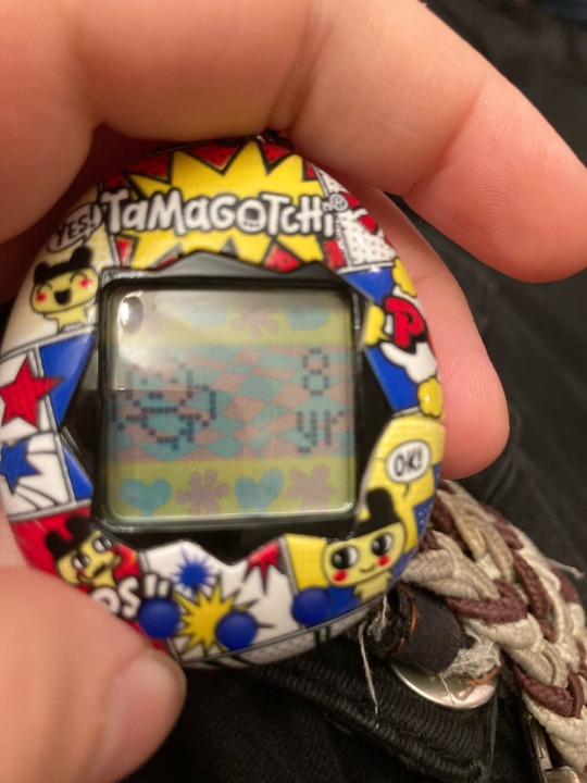
An update on my tamagotchi:
He’s grown up somewhat. Look at my boi. Now he’s an even bigger blob

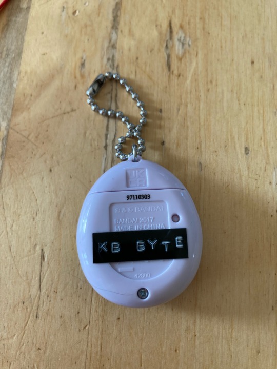
Also I finally decided on a name (with help from my parents and my friend)
Meet KB Byte (short for Knife Bit Byte)
See it’s official:
5 notes
·
View notes
Link
(Via: Lobsters)
By Franck Pachot
.
I’ll reference Alex DeBrie article “SQL, NoSQL, and Scale: How DynamoDB scales where relational databases don’t“, especially the paragraph about “Why relational databases don’t scale”. But I want to make clear that my post here is not against this article, but against a very common myth that even precedes NoSQL databases. Actually, I’m taking this article as reference because the author, in his website and book, has really good points about data modeling in NoSQL. And because AWS DynamoDB is probably the strongest NoSQL database today. I’m challenging some widespread assertions and better do it based on good quality content and product.
There are many use cases where NoSQL is a correct alternative, but moving from a relational database system to a key-value store because you heard that “joins don’t scale” is probably not a good reason. You should choose a solution for the features it offers (the problem it solves), and not because you ignore what you current platform is capable of.
time complexity of joins
The idea in this article, taken from the popular Rick Houlihan talk, is that, by joining tables, you read more data. And that it is a CPU intensive operation. And the time complexity of joins is “( O (M + N) ) or worse” according to Alex DeBrie article or “O(log(N))+Nlog(M)” according to Rick Houlihan slide. This makes reference to “time complexity” and “Big O” notation. You can read about it. But this supposes that the cost of a join depends on the size of the tables involved (represented by N and M). That would be right with non-partitioned table full scan. But all relational databases come with B*Tree indexes. And when we compare to a key-value store we are obviously retrieving few rows and the join method will be a Nested Loop with Index Range Scan. This access method is actually not dependent at all on the size of the tables. That’s why relational database are the king of OTLP applications.
Let’s test it
The article claims that “there’s one big problem with relational databases: performance is like a black box. There are a ton of factors that impact how quickly your queries will return.” with an example on a query like: “SELECT * FROM orders JOIN users ON … WHERE user.id = … GROUP BY … LIMIT 20”. It says that “As the size of your tables grow, these operations will get slower and slower.”
I will build those tables, in PostgreSQL here, because that’s my preferred Open Source RDBMS, and show that:
Performance is not a black box: all RDBMS have an EXPLAIN command that display exactly the algorithm used (even CPU and memory access) and you can estimate the cost easily from it.
Join and Group By here do not depend on the size of the table at all but only the rows selected. You will multiply your tables by several orders of magnitude before the number of rows impact the response time by a 1/10s of millisecond.
Create the tables
I will create small tables here. Because when reading the execution plan, I don’t need large tables to estimate the cost and the response-time scalability. You can run the same with larger tables if you want to see how it scales. And then maybe investigate further the features for big tables (partitioning, parallel query,…). But let’s start with very simple tables without specific optimization.
\timing create table USERS ( USER_ID bigserial primary key, FIRST_NAME text, LAST_NAME text) ; CREATE TABLE create table ORDERS ( ORDER_ID bigserial primary key, ORDER_DATE timestamp, AMOUNT numeric(10,2), USER_ID bigint, DESCRIPTION text) ;
I have created the two tables that I’ll join. Both with an auto-generated primary key for simplicity.
Insert test data
It is important to build the table as they would be in real life. USERS probably come without specific order. ORDERS come by date. This means that ORDERS from one USER are scattered throughout the table. The query would be much faster with clustered data, and each RDBMS has some ways to achieve this, but I want to show the cost of joining two tables here without specific optimisation.
insert into USERS (FIRST_NAME, LAST_NAME) with random_words as ( select generate_series id, translate(md5(random()::text),'-0123456789','aeioughij') as word from generate_series(1,100) ) select words1.word ,words2.word from random_words words1 cross join random_words words2 order by words1.id+words2.id ; INSERT 0 10000 Time: 28.641 ms select * from USERS order by user_id fetch first 10 rows only; user_id | first_name | last_name ---------+--------------------------------+-------------------------------- 1 | iooifgiicuiejiaeduciuccuiogib | iooifgiicuiejiaeduciuccuiogib 2 | iooifgiicuiejiaeduciuccuiogib | dgdfeeiejcohfhjgcoigiedeaubjbg 3 | dgdfeeiejcohfhjgcoigiedeaubjbg | iooifgiicuiejiaeduciuccuiogib 4 | ueuedijchudifefoedbuojuoaudec | iooifgiicuiejiaeduciuccuiogib 5 | iooifgiicuiejiaeduciuccuiogib | ueuedijchudifefoedbuojuoaudec 6 | dgdfeeiejcohfhjgcoigiedeaubjbg | dgdfeeiejcohfhjgcoigiedeaubjbg 7 | iooifgiicuiejiaeduciuccuiogib | jbjubjcidcgugubecfeejidhoigdob 8 | jbjubjcidcgugubecfeejidhoigdob | iooifgiicuiejiaeduciuccuiogib 9 | ueuedijchudifefoedbuojuoaudec | dgdfeeiejcohfhjgcoigiedeaubjbg 10 | dgdfeeiejcohfhjgcoigiedeaubjbg | ueuedijchudifefoedbuojuoaudec (10 rows) Time: 0.384 ms
This generated 10000 users in the USERS table with random names.
insert into ORDERS ( ORDER_DATE, AMOUNT, USER_ID, DESCRIPTION) with random_amounts as ( ------------> this generates 10 random order amounts select 1e6*random() as AMOUNT from generate_series(1,10) ) ,random_dates as ( ------------> this generates 10 random order dates select now() - random() * interval '1 year' as ORDER_DATE from generate_series(1,10) ) select ORDER_DATE, AMOUNT, USER_ID, md5(random()::text) DESCRIPTION from random_dates cross join random_amounts cross join users order by ORDER_DATE ------------> I sort this by date because that's what happens in real life. Clustering by users would not be a fair test. ; INSERT 0 1000000 Time: 4585.767 ms (00:04.586)
I have now one million orders generated as 100 orders for each users in the last year. You can play with the numbers to generate more and see how it scales. This is fast: 5 seconds to generate 1 million orders here, and there are many way to load faster if you feel the need to test on very large data sets. But the point is not there.
create index ORDERS_BY_USER on ORDERS(USER_ID); CREATE INDEX Time: 316.322 ms alter table ORDERS add constraint ORDERS_BY_USER foreign key (USER_ID) references USERS; ALTER TABLE Time: 194.505 ms
As, in my data model, I want to navigate from USERS to ORDERS I add an index for it. And I declare the referential integrity to avoid logical corruptions in case there is a bug in my application, or a human mistake during some ad-hoc fixes. As soon as the constraint is declared, I have no need to check this assertion in my code anymore. The constraint also informs the query planner know about this one-to-many relationship as it may open some optimizations. That’s the relational database beauty: we declare those things rather than having to code their implementation.
vacuum analyze; VACUUM Time: 429.165 ms select version(); version --------------------------------------------------------------------------------------------------------- PostgreSQL 12.3 on x86_64-pc-linux-gnu, compiled by gcc (GCC) 4.8.5 20150623 (Red Hat 4.8.5-39), 64-bit (1 row)
I’m in PostgreSQL, version 12, on a Linux box with 2 CPUs only. I’ve run a manual VACUUM to get a reproducible testcase rather than relying on autovacuum kicking-in after those table loading.
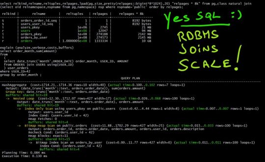
select relkind,relname,reltuples,relpages,lpad(pg_size_pretty(relpages::bigint*8*1024),20) "relpages * 8k" from pg_class natural join (select oid relnamespace,nspname from pg_namespace) nsp where nspname='public' order by relpages; relkind | relname | reltuples | relpages | relpages * 8k ---------+---------------------+-----------+----------+---------------------- S | orders_order_id_seq | 1 | 1 | 8192 bytes S | users_user_id_seq | 1 | 1 | 8192 bytes i | users_pkey | 10000 | 30 | 240 kB r | users | 10000 | 122 | 976 kB i | orders_pkey | 1e+06 | 2745 | 21 MB i | orders_by_user | 1e+06 | 2749 | 21 MB r | orders | 1e+06 | 13334 | 104 MB
Here are the sizes of my tables: The 1 million orders take 104MB and the 10 thousand users is 1MB. I’ll increase it later, but I don’t need this to understand the performance predictability.
When understanding the size, remember that the size of the table is only the size of data. Metadata (like column names) are not repeated for each row. They are stored once in the RDBMS catalog describing the table. As PostgreSQL has a native JSON datatype you can also test with a non-relational model here.
Execute the query
select order_month,sum(amount),count(*) from ( select date_trunc('month',ORDER_DATE) order_month, USER_ID, AMOUNT from ORDERS join USERS using(USER_ID) ) user_orders where USER_ID=42 group by order_month ; order_month | sum | count ---------------------+-------------+------- 2019-11-01 00:00:00 | 5013943.57 | 10 2019-09-01 00:00:00 | 5013943.57 | 10 2020-04-01 00:00:00 | 5013943.57 | 10 2019-08-01 00:00:00 | 15041830.71 | 30 2020-02-01 00:00:00 | 10027887.14 | 20 2020-06-01 00:00:00 | 5013943.57 | 10 2019-07-01 00:00:00 | 5013943.57 | 10 (7 rows) Time: 2.863 ms
Here is the query mentioned in the article: get all orders for one user, and do some aggregation on them. Looking at the time is not really interesting as it depends on the RAM to cache the buffers at database or filesystem level, and disk latency. But we are developers and, by looking at the operations and loops that were executed, we can understand how it scales and where we are in the “time complexity” and “Big O” order of magnitude.
Explain the execution
This is as easy as running the query with EXPLAIN:
explain (analyze,verbose,costs,buffers) select order_month,sum(amount) from ( select date_trunc('month',ORDER_DATE) order_month, USER_ID, AMOUNT from ORDERS join USERS using(USER_ID) ) user_orders where USER_ID=42 group by order_month ; QUERY PLAN ------------------------------------------------------------------------------------------------------------------------------------------------ GroupAggregate (cost=389.34..390.24 rows=10 width=40) (actual time=0.112..0.136 rows=7 loops=1) Output: (date_trunc('month'::text, orders.order_date)), sum(orders.amount) Group Key: (date_trunc('month'::text, orders.order_date)) Buffers: shared hit=19 -> Sort (cost=389.34..389.59 rows=100 width=17) (actual time=0.104..0.110 rows=100 loops=1) Output: (date_trunc('month'::text, orders.order_date)), orders.amount Sort Key: (date_trunc('month'::text, orders.order_date)) Sort Method: quicksort Memory: 32kB Buffers: shared hit=19 -> Nested Loop (cost=5.49..386.02 rows=100 width=17) (actual time=0.022..0.086 rows=100 loops=1) Output: date_trunc('month'::text, orders.order_date), orders.amount Buffers: shared hit=19 -> Index Only Scan using users_pkey on public.users (cost=0.29..4.30 rows=1 width=8) (actual time=0.006..0.006 rows=1 loops=1) Output: users.user_id Index Cond: (users.user_id = 42) Heap Fetches: 0 Buffers: shared hit=3 -> Bitmap Heap Scan on public.orders (cost=5.20..380.47 rows=100 width=25) (actual time=0.012..0.031 rows=100 loops=1) Output: orders.order_id, orders.order_date, orders.amount, orders.user_id, orders.description Recheck Cond: (orders.user_id = 42) Heap Blocks: exact=13 Buffers: shared hit=16 -> Bitmap Index Scan on orders_by_user (cost=0.00..5.17 rows=100 width=0) (actual time=0.008..0.008 rows=100 loops=1) Index Cond: (orders.user_id = 42) Buffers: shared hit=3 Planning Time: 0.082 ms Execution Time: 0.161 ms
Here is the execution plan with the execution statistics. We have read 3 pages from USERS to get our USER_ID (Index Only Scan) and navigated, with Nested Loop, to ORDERS and get the 100 orders for this user. This has read 3 pages from the index (Bitmap Index Scan) and 13 pages from the table. That’s a total of 19 pages. Those pages are 8k blocks.
4x initial size scales with same performance: 19 page reads
Let’s increase the size of the tables by a factor 4. I change the “generate_series(1,100)” to “generate_series(1,200)” in the USERS generations and run the same. That generates 40000 users and 4 million orders.
select relkind,relname,reltuples,relpages,lpad(pg_size_pretty(relpages::bigint*8*1024),20) "relpages * 8k" from pg_class natural join (select oid relnamespace,nspname from pg_namespace) nsp where nspname='public' order by relpages; relkind | relname | reltuples | relpages | relpages * 8k ---------+---------------------+--------------+----------+---------------------- S | orders_order_id_seq | 1 | 1 | 8192 bytes S | users_user_id_seq | 1 | 1 | 8192 bytes i | users_pkey | 40000 | 112 | 896 kB r | users | 40000 | 485 | 3880 kB i | orders_pkey | 4e+06 | 10969 | 86 MB i | orders_by_user | 4e+06 | 10985 | 86 MB r | orders | 3.999995e+06 | 52617 | 411 MB explain (analyze,verbose,costs,buffers) select order_month,sum(amount) from ( select date_trunc('month',ORDER_DATE) order_month, USER_ID, AMOUNT from ORDERS join USERS using(USER_ID) ) user_orders where USER_ID=42 group by order_month ; explain (analyze,verbose,costs,buffers) select order_month,sum(amount) from ( select date_trunc('month',ORDER_DATE) order_month, USER_ID, AMOUNT from ORDERS join USERS using(USER_ID) ) user_orders where USER_ID=42 group by order_month ; QUERY PLAN ------------------------------------------------------------------------------------------------------------------------------------------------ GroupAggregate (cost=417.76..418.69 rows=10 width=40) (actual time=0.116..0.143 rows=9 loops=1) Output: (date_trunc('month'::text, orders.order_date)), sum(orders.amount) Group Key: (date_trunc('month'::text, orders.order_date)) Buffers: shared hit=19 -> Sort (cost=417.76..418.02 rows=104 width=16) (actual time=0.108..0.115 rows=100 loops=1) Output: (date_trunc('month'::text, orders.order_date)), orders.amount Sort Key: (date_trunc('month'::text, orders.order_date)) Sort Method: quicksort Memory: 32kB Buffers: shared hit=19 -> Nested Loop (cost=5.53..414.27 rows=104 width=16) (actual time=0.044..0.091 rows=100 loops=1) Output: date_trunc('month'::text, orders.order_date), orders.amount Buffers: shared hit=19 -> Index Only Scan using users_pkey on public.users (cost=0.29..4.31 rows=1 width=8) (actual time=0.006..0.007 rows=1 loops=1) Output: users.user_id Index Cond: (users.user_id = 42) Heap Fetches: 0 Buffers: shared hit=3 -> Bitmap Heap Scan on public.orders (cost=5.24..408.66 rows=104 width=24) (actual time=0.033..0.056 rows=100 loops=1) Output: orders.order_id, orders.order_date, orders.amount, orders.user_id, orders.description Recheck Cond: (orders.user_id = 42) Heap Blocks: exact=13 Buffers: shared hit=16 -> Bitmap Index Scan on orders_by_user (cost=0.00..5.21 rows=104 width=0) (actual time=0.029..0.029 rows=100 loops=1) Index Cond: (orders.user_id = 42) Buffers: shared hit=3 Planning Time: 0.084 ms Execution Time: 0.168 ms (27 rows) Time: 0.532 ms
Look how we scaled here: I multiplied the size of the tables by 4x and I have exactly the same cost: 3 pages from each index and 13 from the table. This is the beauty of B*Tree: the cost depends only on the height of the tree and not the size of the table. And you can increase the table exponentially before the height of the index increases.
16x initial size scales with 21/19=1.1 cost factor
Let’s go further and x4 the size of the tables again. I run with “generate_series(1,400)” in the USERS generations and run the same. That generates 160 thousand users and 16 million orders.
select relkind,relname,reltuples,relpages,lpad(pg_size_pretty(relpages::bigint*8*1024),20) "relpages * 8k" from pg_class natural join (select oid relnamespace,nspname from pg_namespace) nsp where nspname='public' order by relpages; relkind | relname | reltuples | relpages | relpages * 8k ---------+---------------------+--------------+----------+---------------------- S | orders_order_id_seq | 1 | 1 | 8192 bytes S | users_user_id_seq | 1 | 1 | 8192 bytes i | users_pkey | 160000 | 442 | 3536 kB r | users | 160000 | 1925 | 15 MB i | orders_pkey | 1.6e+07 | 43871 | 343 MB i | orders_by_user | 1.6e+07 | 43935 | 343 MB r | orders | 1.600005e+07 | 213334 | 1667 MB explain (analyze,verbose,costs,buffers) select order_month,sum(amount) from ( select date_trunc('month',ORDER_DATE) order_month, USER_ID, AMOUNT from ORDERS join USERS using(USER_ID) ) user_orders where USER_ID=42 group by order_month ; QUERY PLAN ------------------------------------------------------------------------------------------------------------------------------------------------ GroupAggregate (cost=567.81..569.01 rows=10 width=40) (actual time=0.095..0.120 rows=8 loops=1) Output: (date_trunc('month'::text, orders.order_date)), sum(orders.amount) Group Key: (date_trunc('month'::text, orders.order_date)) Buffers: shared hit=21 -> Sort (cost=567.81..568.16 rows=140 width=17) (actual time=0.087..0.093 rows=100 loops=1) Output: (date_trunc('month'::text, orders.order_date)), orders.amount Sort Key: (date_trunc('month'::text, orders.order_date)) Sort Method: quicksort Memory: 32kB Buffers: shared hit=21 -> Nested Loop (cost=6.06..562.82 rows=140 width=17) (actual time=0.026..0.070 rows=100 loops=1) Output: date_trunc('month'::text, orders.order_date), orders.amount Buffers: shared hit=21 -> Index Only Scan using users_pkey on public.users (cost=0.42..4.44 rows=1 width=8) (actual time=0.007..0.007 rows=1 loops=1) Output: users.user_id Index Cond: (users.user_id = 42) Heap Fetches: 0 Buffers: shared hit=4 -> Bitmap Heap Scan on public.orders (cost=5.64..556.64 rows=140 width=25) (actual time=0.014..0.035 rows=100 loops=1) Output: orders.order_id, orders.order_date, orders.amount, orders.user_id, orders.description Recheck Cond: (orders.user_id = 42) Heap Blocks: exact=13 Buffers: shared hit=17 -> Bitmap Index Scan on orders_by_user (cost=0.00..5.61 rows=140 width=0) (actual time=0.010..0.010 rows=100 loops=1) Index Cond: (orders.user_id = 42) Buffers: shared hit=4 Planning Time: 0.082 ms Execution Time: 0.159 ms
Yes, by increasing the table size a lot the index may have to split the root block to add a new branch level. The consequence is minimal: two additional pages to read here. The additional execution time is in tens of microseconds when cached in RAM, up to milliseconds if from mechanical disk. With 10x or 100x larger tables, you will do some physical I/O and only the top index branches will be in memory. You can expect about about 20 I/O calls then. With SSD on Fiber Channel (like with AWS RDS PostgreSQL for example), this will still be in single-digit millisecond. The cheapest AWS EBS Provisioned IOPS for RDS is 1000 IOPS then you can estimate the number of queries per second you can run. The number of pages here (“Buffers”) is the right metric to estimate the cost of the query. To be compared with DynamoDB RCU.
64x initial size scales with 23/19=1.2 cost factor
Last test for me, but you can go further, I change to “generate_series(1,800)” in the USERS generations and run the same. That generates 640 thousand users and 64 million orders.
select relkind,relname,reltuples,relpages,lpad(pg_size_pretty(relpages::bigint*8*1024),20) "relpages * 8k" from pg_class natural join (select oid relnamespace,nspname from pg_namespace) nsp where nspname='public' order by relpages; relkind | relname | reltuples | relpages | relpages * 8k ---------+---------------------+---------------+----------+---------------------- S | orders_order_id_seq | 1 | 1 | 8192 bytes S | users_user_id_seq | 1 | 1 | 8192 bytes i | users_pkey | 640000 | 1757 | 14 MB r | users | 640000 | 7739 | 60 MB i | orders_pkey | 6.4e+07 | 175482 | 1371 MB i | orders_by_user | 6.4e+07 | 175728 | 1373 MB r | orders | 6.4000048e+07 | 853334 | 6667 MB explain (analyze,verbose,costs,buffers) select order_month,sum(amount) from ( select date_trunc('month',ORDER_DATE) order_month, USER_ID, AMOUNT from ORDERS join USERS using(USER_ID) ) user_orders where USER_ID=42 group by order_month ; QUERY PLAN ------------------------------------------------------------------------------------------------------------------------------------------ HashAggregate (cost=1227.18..1227.33 rows=10 width=40) (actual time=0.102..0.105 rows=7 loops=1) Output: (date_trunc('month'::text, orders.order_date)), sum(orders.amount) Group Key: date_trunc('month'::text, orders.order_date) Buffers: shared hit=23 -> Nested Loop (cost=7.36..1225.65 rows=306 width=17) (actual time=0.027..0.072 rows=100 loops=1) Output: date_trunc('month'::text, orders.order_date), orders.amount Buffers: shared hit=23 -> Index Only Scan using users_pkey on public.users (cost=0.42..4.44 rows=1 width=8) (actual time=0.007..0.008 rows=1 loops=1) Output: users.user_id Index Cond: (users.user_id = 42) Heap Fetches: 0 Buffers: shared hit=4 -> Bitmap Heap Scan on public.orders (cost=6.94..1217.38 rows=306 width=25) (actual time=0.015..0.037 rows=100 loops=1) Output: orders.order_id, orders.order_date, orders.amount, orders.user_id, orders.description Recheck Cond: (orders.user_id = 42) Heap Blocks: exact=15 Buffers: shared hit=19 -> Bitmap Index Scan on orders_by_user (cost=0.00..6.86 rows=306 width=0) (actual time=0.011..0.011 rows=100 loops=1) Index Cond: (orders.user_id = 42) Buffers: shared hit=4 Planning Time: 0.086 ms Execution Time: 0.134 ms (22 rows) Time: 0.521 ms
You see how the cost increases slowly, with two additional pages to read here.
Please, test with more rows. When looking at the time (less than 1 millisecond), keep in mind that it is CPU time here as all pages are in memory cache. On purpose, because the article mentions CPU and RAM (“joins require a lot of CPU and memory”). Anyway, 20 disk reads will still be within the millisecond on modern storage.
Time complexity of B*Tree is actually very light
Let’s get back to the “Big O” notation. We are definitely not “O (M + N)”. This would have been without any index, where all pages from all tables would have been full scanned. Any database maintains hashed or sorted structures to improve high selectivity queries. This has nothing to do with SQL vs. NoSQL or with RDBMS vs. Hierarchichal DB. In DynamoDB this structure on primary key is HASH partitioning (and additional sorting). In RDBMS the most common structure is a sorted index (with the possibility of additional partitioning, zone maps, clustering,…). We are not in “O(log(N))+Nlog(M)” but more like “O(log(N))+log(M)” because the size of the driving table (N) has nothing to do on the inner loop cost. The first filtering, the one with “O(log(N))”, has filtered out those N rows. Using “N” and ignoring the outer selectivity is a mistake. Anyway, this O(log) for B*Tree is really scalable as we have seen because the base of this log() function is really small (thanks to large branch blocks – 8KB).
Anyway, the point is not there. As you have seen, the cost of Nested Loop is in the blocks that are fetched from the inner loop, and this depends on the selectivity and the clustering factor (the table physical order correlation with the index order), and some prefetching techniques. This O(log) for going through the index is often insignificant on Range Scans.
40 years of RDBMS optimizations
If you have a database size that is several order of magnitude from those million rows, and where this millisecond latency is a problem, the major RDBMS offer many features and structures to go further in performance and predictability of response time. As we have seen, the cost of this query is not about Index, Nested Loop or Group By. It is about the scattered items: ingested by date but queried by user.
Through its 40 years of optimizing OLTP applications, the Oracle Database have a lot of features, with their popularity depending on the IT trends. From the first versions, in the 80’s, because the hierarchical databases were still in people’s mind, and the fear of “joins are expensive” was already there, Oracle has implemented a structure to store the tables together, pre-joined. This is called CLUSTER. It was, from the beginning, indexed with a sorted structure (INDEX CLUSTER) or a hashed structure (HASH CLUSTER). Parallel Query was quickly implemented to scale-up and, with Parallel Server now known as RAC, to scale-out. Partitioning was introduced to scale further, again with sorted (PARTITION by RANGE) or hashed (PARTITION BY HASH) segments. This can scale further the index access (LOCAL INDEX with partition pruning). And it also scales joins (PARTITION-WISE JOIN) to reduce CPU and RAM to join large datasets. When more agility was needed, B*Tree sorted structures were the winner and Index Organized Tables were introduced to cluster data (to avoid the most expensive operation as we have seen in the examples above). But Heap Tables and B*Tree are still the winners given their agility and because the Join operations were rarely a bottleneck. Currently, partitioning has improved (even scaling horizontally beyond the clusters with sharding), as well as data clustering (Attribute Clustering, Zone Maps and Storage Index). And there’s always the possibility for Index Only access, just by adding more columns to the index, removing the major cost of table access. And materialized views can also act as pre-built join index and will also reduce the CPU and RAM required for GROUP BY aggregation.
I listed a lot of Oracle features, but Microsoft SQL Server has also many similar features. Clustered tables, covering indexes, Indexed Views, and of course partitioning. Open source databases are evolving a lot. PostgreSQL has partitioning, parallel query, clustering,.. Still Open Source, you can web-scale it to a distributed database with YugabyteDB. MySQL is evolving a lot recently. I’ll not list all databases and all features. You can port the testcase to other databases easily.
Oh, and by the way, if you want to test it on Oracle Database you will quickly realize that the query from the article may not even do any Join operation. Because when you query with the USER_ID you probably don’t need to get back to the USERS table. And thanks to the declared foreign key, the optimizer knows that the join is not necessary: https://dbfiddle.uk/?rdbms=oracle_18&fiddle=a5afeba2fdb27dec7533545ab0a6eb0e.
NoSQL databases are good for many use-cases. But remember that it is a key-value optimized data store. When you start to split a document into multiple entities with their own keys, remember that relational databases were invented for that. I blogged about another myth recently: The myth of NoSQL (vs. RDBMS) agility: adding attributes. All feedback welcome, here or on Twitter:
0 notes
Text
How I Used Brotli to Get Even Smaller CSS and JavaScript Files at CDN Scale
The HBO sitcom Silicon Valley hilariously followed Pied Piper, a team of developers with startup dreams to create a compression algorithm so powerful that high-quality streaming and file storage concerns would become a thing of the past.

In the show, Google is portrayed by the fictional company Hooli, which is after Pied Piper’s intellectual property. The funny thing is that, while being far from a startup, Google does indeed have a powerful compression engine in real life called Brotli.
This article is about my experience using Brotli at production scale. Despite being really expensive and a truly unfeasible method for on-the-fly compression, Brotli is actually very economical and saves cost on many fronts, especially when compared with gzip or lower compression levels of Brotli (which we’ll get into).
Brotli’s beginning…
In 2015, Google published a blog post announcing Brotli and released its source code on GitHub. The pair of developers who created Brotli also created Google’s Zopfli compression two years earlier. But where Zopfli leveraged existing compression techniques, Brotli was written from the ground-up and squarely focused on text compression to benefit static web assets, like HTML, CSS, JavaScript and even web fonts.
At that time, I was working as a freelance website performance consultant. I was really excited for the 20-26% improvement Brotli promised over Zopfli. Zopfli in itself is a dense implementation of the deflate compressor compared with zlib’s standard implementation, so the claim of up to 26% was quite impressive. And what’s zlib? It’s essentially the same as gzip.
So what we’re looking at is the next generation of Zopfli, which is an offshoot of zlib, which is essentially gzip.
A story of disappointment
It took a few months for major CDN players to support Brotli, but meanwhile it was seeing widespread adoption in tools, services, browsers and servers. However, the 26% dense compression that Brotli promised was never reflected in production. Some CDNs set a lower compression level internally while others supported Brotli at origin so that they only support it if it was enabled manually at the origin.
Server support for Brotli was pretty good, but to achieve high compression levels, it required rolling your own pre-compression code or using a server module to do it for you — which is not always an option, especially in the case of shared hosting services.
This was really disappointing for me. I wanted to compress every last possible byte for my clients’ websites in a drive to make them faster, but using pre-compression and allowing clients to update files on demand simultaneously was not always easy.
Taking matters into my own hands
I started building my own performance optimization service for my clients.
I had several tricks that could significantly speed up websites. The service categorized all the optimizations in three groups consisting of several “Content,” “Delivery,” and “Cache” optimizations. I had Brotli in mind for the content optimization part of the service for compressible resources.
Like other compression formats, Brotli comes in different levels of power. Brotli’s max level is exactly like the max volume of the guitar amps in This is Spinal Tap: it goes to 11.
youtube
Brotli:11, or Brotli compression level 11, can offer significant reduction in the size of compressible files, but has a substantial trade-off: it is painfully slow and not feasible for on demand compression the same way gzip is capable of doing it. It costs significantly more in terms of CPU time.
In my benchmarks, Brotli:11 takes several hundred milliseconds to compress a single minified jQuery file. So, the only way to offer Brotli:11 to my clients was to use it for pre-compression, leaving me to figure out a way to cache files at the server level. Luckily we already had that in place. The only problem was the fear that Brotli could kill all our processing resources.

Maybe that’s why Pied Piper had to continue rigging its servers for more power.
I put my fears aside and built Brotli:11 as a configurable server option. This way, clients could decide whether enabling it was worth the computing cost.
It’s slow, but gradually pays off
Among several other optimizations, the service for my clients also offers geographic content delivery; in other words, it has a built-in CDN.
Of the several tricks I tried when taking matters into my own hands, one was to combine public CDN (or open-source CDN) and private CDN on a single host so that websites can enjoy the benefits of shared browser cache of public resources without incurring separate DNS lookup and connection cost for that public host. I wanted to avoid this extra connection cost because it has significant impact for mobile users. Also, combining more and more resources on a single host can help get the most of HTTP/2 features, like multiplexing.
I enabled the public CDN and turned on Brotli:11 pre-compression for all compressible resources, including CSS, JavaScript, SVG, and TTF, among other types of files. The overhead of compression did indeed increase on first request of each resource — but after that, everything seemed to run smoothly. Brotli has over 90% browser support and pretty much all the requests hitting my service now use Brotli.
I was happy. Clients were happy. But I didn’t have numbers. I started analyzing the impact of enabling this high density compression on public resources. For this, I recorded file transfer sizes of several popular libraries — including jQuery, Bootstrap, React, and other frameworks — that used common compression methods implemented by other CDNs and found that Brotli:11 compression was saving around 21% compared to other compression formats.
It’s important to note that some of the other public CDNs I compared were already using Brotli, but at lower compression levels. So, the 21% extra compression was really satisfying for me. This number is based on a very small subset of libraries but is not incorrect by a big margin as I was seeing this much gain on all of the websites that I tested.
Here is a graphical representation of the savings.

You can see the raw data below..Note that the savings for CSS is much more prominent than what JavaScript gets.
LibraryOriginalAvg. of Common Compression (A)Brotli:11 (B)(A) / (B) – 1Ant Design1,938.99 KB438.24 KB362.82 KB20.79%Bootstrap152.11 KB24.20 KB17.30 KB39.88%Bulma186.13 KB23.40 KB19.30 KB21.24%D3.js236.82 KB74.51 KB65.75 KB13.32%Font Awesome1,104.04 KB422.56 KB331.12 KB27.62%jQuery86.08 KB30.31 KB27.65 KB9.62%React105.47 KB33.33 KB30.28 KB10.07%Semantic UI613.78 KB91.93 KB78.25 KB17.48%three.js562.75 KB134.01 KB114.44 KB17.10%Vue.js91.48 KB33.17 KB30.58 KB8.47%
The results are great, which is what I expected. But what about the overall impact of using Brotli:11 at scale? Turns out that using Brotli:11 for all public resources reduces cost all around:
The smaller file sizes are expected to result in lower TLS overhead. That said, it is not easily measurable, nor is it significant for my service because modern CPUs are very fast at encryption. Still, I believe there is some tiny and repeated saving on account of encryption for every request as smaller files encrypt faster.
It reduces the bandwidth cost. The 21% savings I got across the board is the case in point. And, remember, savings are not a one-time thing. Each request counts as cost, so the 21% savings is repeated time and again, creating a snowball savings for the cost of bandwidth.
We only cache hot files in memory at edge servers. Due to the widespread browser support for Brotli, these hot files are mostly encoded by Brotli and their small size lets us fit more of them in available memory.
Visitors, especially those on mobile devices, enjoy reduced data transfer. This results in less battery use and savings on data charges. That’s a huge win that gets passed on to the users of our clients!
This is all so good. The cost we save per request is not significant, but considering we have a near zero cache miss rate for public resources, we can easily amortize the initial high cost of compression in next several hundred requests. After that, we’re looking at a lifetime benefit of reduced overhead.
It doesn’t end there
With the mix of public and private CDNs that we introduced as part of our performance optimization service, we wanted to make sure that clients could set lower compression levels for resources that frequently change over time (like custom CSS and JavaScript) on the private CDN and automatically switch to the public CDN for open-source resources that change less often and have pre-configured Brotli:11. This way, our clients can still get a high compression ratio on resources that change less often while still enjoying good compression ratios with instant purge and updates for compressible resources.
This all is done smoothly and seamlessly using our integration tools. The added benefit of this approach for clients is that the bandwidth on the public CDN is totally free with unprecedented performance levels.
Try it yourself!
Testing on a common website, using aggressive compression can easily shave around 50 KB off the page load. If you want to play with the free public CDN and enjoy smaller CSS and JavaScript, you are welcome to use our PageCDN service. Here are some of the most used libraries for your use:
<!-- jQuery 3.5.0 --> <script src="https://pagecdn.io/lib/jquery/3.5.0/jquery.min.js" crossorigin="anonymous" integrity="sha256-xNzN2a4ltkB44Mc/Jz3pT4iU1cmeR0FkXs4pru/JxaQ=" ></script>
<!-- FontAwesome 5.13.0 --> <link href="https://pagecdn.io/lib/font-awesome/5.13.0/css/all.min.css" rel="stylesheet" crossorigin="anonymous" integrity="sha256-h20CPZ0QyXlBuAw7A+KluUYx/3pK+c7lYEpqLTlxjYQ=" >
<!-- Ionicons 4.6.3 --> <link href="https://pagecdn.io/lib/ionicons/4.6.3/css/ionicons.min.css" rel="stylesheet" crossorigin="anonymous" integrity="sha256-UUDuVsOnvDZHzqNIznkKeDGtWZ/Bw9ZlW+26xqKLV7c=" >
<!-- Bootstrap 4.4.1 --> <link href="https://pagecdn.io/lib/bootstrap/4.4.1/css/bootstrap.min.css" rel="stylesheet" crossorigin="anonymous" integrity="sha256-L/W5Wfqfa0sdBNIKN9cG6QA5F2qx4qICmU2VgLruv9Y=" >
<!-- React 16.13.1 --> <script src="https://pagecdn.io/lib/react/16.13.1/umd/react.production.min.js" crossorigin="anonymous" integrity="sha256-yUhvEmYVhZ/GGshIQKArLvySDSh6cdmdcIx0spR3UP4=" ></script>
<!-- Vue 2.6.11 --> <script src="https://pagecdn.io/lib/vue/2.6.11/vue.min.js" crossorigin="anonymous" integrity="sha256-ngFW3UnAN0Tnm76mDuu7uUtYEcG3G5H1+zioJw3t+68=" ></script>
Our PHP library automatic switches between private and public CDN if you need it to. The same feature is implemented seamlessly in our WordPress plugin that automatically loads public resources over Public CDN. Both of these tools allow full access to the free public CDN. Libraries for JavaScript, Python. and Ruby are not yet available. If you contribute any such library to our Public CDN, I will be happy to list it in our docs.
Additionally, you can use our search tool to immediately find a corresponding resource on the public CDN by supplying a URL of a resource on your website. If none of these tools work for you, then you can check the relevant library page and pick the URLs you want.
Looking toward the future
We started by hosting only the most popular libraries in order to prevent malware spread. However, things are changing rapidly and we add new libraries as our users suggest them to us. You are welcome to suggest your favorite ones, too. If you still want to link to a public or private Github repo that is not yet available on our public CDN, you can use our private CDN to connect to a repo and import all new releases as they appear on GitHub and then apply your own aggressive optimizations before delivery.
What do you think?
Everything we covered here is solely based on my personal experience working with Brotli compression at CDN scale. It just happens to be an introduction to my public CDN as well. We are still a small service and our client websites are only in the hundreds. Still, at this scale the aggressive compression seems to pay off.
I achieved high quality results for my clients and now you can use this free service for your websites as well. And, if you like it, please leave feedback at my email and recommend it to others.
The post How I Used Brotli to Get Even Smaller CSS and JavaScript Files at CDN Scale appeared first on CSS-Tricks.
How I Used Brotli to Get Even Smaller CSS and JavaScript Files at CDN Scale published first on https://deskbysnafu.tumblr.com/
0 notes
Text
How I Used Brotli to Get Even Smaller CSS and JavaScript Files at CDN Scale
The HBO sitcom Silicon Valley hilariously followed Pied Piper, a team of developers with startup dreams to create a compression algorithm so powerful that high-quality streaming and file storage concerns would become a thing of the past.

In the show, Google is portrayed by the fictional company Hooli, which is after Pied Piper’s intellectual property. The funny thing is that, while being far from a startup, Google does indeed have a powerful compression engine in real life called Brotli.
This article is about my experience using Brotli at production scale. Despite being really expensive and a truly unfeasible method for on-the-fly compression, Brotli is actually very economical and saves cost on many fronts, especially when compared with gzip or lower compression levels of Brotli (which we’ll get into).
Brotli’s beginning…
In 2015, Google published a blog post announcing Brotli and released its source code on GitHub. The pair of developers who created Brotli also created Google’s Zopfli compression two years earlier. But where Zopfli leveraged existing compression techniques, Brotli was written from the ground-up and squarely focused on text compression to benefit static web assets, like HTML, CSS, JavaScript and even web fonts.
At that time, I was working as a freelance website performance consultant. I was really excited for the 20-26% improvement Brotli promised over Zopfli. Zopfli in itself is a dense implementation of the deflate compressor compared with zlib’s standard implementation, so the claim of up to 26% was quite impressive. And what’s zlib? It’s essentially the same as gzip.
So what we’re looking at is the next generation of Zopfli, which is an offshoot of zlib, which is essentially gzip.
A story of disappointment
It took a few months for major CDN players to support Brotli, but meanwhile it was seeing widespread adoption in tools, services, browsers and servers. However, the 26% dense compression that Brotli promised was never reflected in production. Some CDNs set a lower compression level internally while others supported Brotli at origin so that they only support it if it was enabled manually at the origin.
Server support for Brotli was pretty good, but to achieve high compression levels, it required rolling your own pre-compression code or using a server module to do it for you — which is not always an option, especially in the case of shared hosting services.
This was really disappointing for me. I wanted to compress every last possible byte for my clients’ websites in a drive to make them faster, but using pre-compression and allowing clients to update files on demand simultaneously was not always easy.
Taking matters into my own hands
I started building my own performance optimization service for my clients.
I had several tricks that could significantly speed up websites. The service categorized all the optimizations in three groups consisting of several “Content,” “Delivery,” and “Cache” optimizations. I had Brotli in mind for the content optimization part of the service for compressible resources.
Like other compression formats, Brotli comes in different levels of power. Brotli’s max level is exactly like the max volume of the guitar amps in This is Spinal Tap: it goes to 11.
youtube
Brotli:11, or Brotli compression level 11, can offer significant reduction in the size of compressible files, but has a substantial trade-off: it is painfully slow and not feasible for on demand compression the same way gzip is capable of doing it. It costs significantly more in terms of CPU time.
In my benchmarks, Brotli:11 takes several hundred milliseconds to compress a single minified jQuery file. So, the only way to offer Brotli:11 to my clients was to use it for pre-compression, leaving me to figure out a way to cache files at the server level. Luckily we already had that in place. The only problem was the fear that Brotli could kill all our processing resources.

Maybe that’s why Pied Piper had to continue rigging its servers for more power.
I put my fears aside and built Brotli:11 as a configurable server option. This way, clients could decide whether enabling it was worth the computing cost.
It’s slow, but gradually pays off
Among several other optimizations, the service for my clients also offers geographic content delivery; in other words, it has a built-in CDN.
Of the several tricks I tried when taking matters into my own hands, one was to combine public CDN (or open-source CDN) and private CDN on a single host so that websites can enjoy the benefits of shared browser cache of public resources without incurring separate DNS lookup and connection cost for that public host. I wanted to avoid this extra connection cost because it has significant impact for mobile users. Also, combining more and more resources on a single host can help get the most of HTTP/2 features, like multiplexing.
I enabled the public CDN and turned on Brotli:11 pre-compression for all compressible resources, including CSS, JavaScript, SVG, and TTF, among other types of files. The overhead of compression did indeed increase on first request of each resource — but after that, everything seemed to run smoothly. Brotli has over 90% browser support and pretty much all the requests hitting my service now use Brotli.
I was happy. Clients were happy. But I didn’t have numbers. I started analyzing the impact of enabling this high density compression on public resources. For this, I recorded file transfer sizes of several popular libraries — including jQuery, Bootstrap, React, and other frameworks — that used common compression methods implemented by other CDNs and found that Brotli:11 compression was saving around 21% compared to other compression formats.
It’s important to note that some of the other public CDNs I compared were already using Brotli, but at lower compression levels. So, the 21% extra compression was really satisfying for me. This number is based on a very small subset of libraries but is not incorrect by a big margin as I was seeing this much gain on all of the websites that I tested.
Here is a graphical representation of the savings.
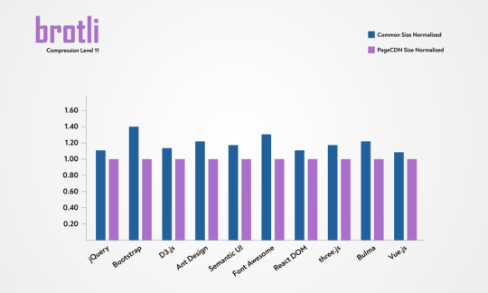
You can see the raw data below..Note that the savings for CSS is much more prominent than what JavaScript gets.
Library Original Avg. of Common Compression (A) Brotli:11 (B) (A) / (B) – 1 Ant Design 1,938.99 KB 438.24 KB 362.82 KB 20.79% Bootstrap 152.11 KB 24.20 KB 17.30 KB 39.88% Bulma 186.13 KB 23.40 KB 19.30 KB 21.24% D3.js 236.82 KB 74.51 KB 65.75 KB 13.32% Font Awesome 1,104.04 KB 422.56 KB 331.12 KB 27.62% jQuery 86.08 KB 30.31 KB 27.65 KB 9.62% React 105.47 KB 33.33 KB 30.28 KB 10.07% Semantic UI 613.78 KB 91.93 KB 78.25 KB 17.48% three.js 562.75 KB 134.01 KB 114.44 KB 17.10% Vue.js 91.48 KB 33.17 KB 30.58 KB 8.47%
The results are great, which is what I expected. But what about the overall impact of using Brotli:11 at scale? Turns out that using Brotli:11 for all public resources reduces cost all around:
The smaller file sizes are expected to result in lower TLS overhead. That said, it is not easily measurable, nor is it significant for my service because modern CPUs are very fast at encryption. Still, I believe there is some tiny and repeated saving on account of encryption for every request as smaller files encrypt faster.
It reduces the bandwidth cost. The 21% savings I got across the board is the case in point. And, remember, savings are not a one-time thing. Each request counts as cost, so the 21% savings is repeated time and again, creating a snowball savings for the cost of bandwidth.
We only cache hot files in memory at edge servers. Due to the widespread browser support for Brotli, these hot files are mostly encoded by Brotli and their small size lets us fit more of them in available memory.
Visitors, especially those on mobile devices, enjoy reduced data transfer. This results in less battery use and savings on data charges. That’s a huge win that gets passed on to the users of our clients!
This is all so good. The cost we save per request is not significant, but considering we have a near zero cache miss rate for public resources, we can easily amortize the initial high cost of compression in next several hundred requests. After that, we’re looking at a lifetime benefit of reduced overhead.
It doesn’t end there
With the mix of public and private CDNs that we introduced as part of our performance optimization service, we wanted to make sure that clients could set lower compression levels for resources that frequently change over time (like custom CSS and JavaScript) on the private CDN and automatically switch to the public CDN for open-source resources that change less often and have pre-configured Brotli:11. This way, our clients can still get a high compression ratio on resources that change less often while still enjoying good compression ratios with instant purge and updates for compressible resources.
This all is done smoothly and seamlessly using our integration tools. The added benefit of this approach for clients is that the bandwidth on the public CDN is totally free with unprecedented performance levels.
Try it yourself!
Testing on a common website, using aggressive compression can easily shave around 50 KB off the page load. If you want to play with the free public CDN and enjoy smaller CSS and JavaScript, you are welcome to use our PageCDN service. Here are some of the most used libraries for your use:
<!-- jQuery 3.5.0 --> <script src="https://pagecdn.io/lib/jquery/3.5.0/jquery.min.js" crossorigin="anonymous" integrity="sha256-xNzN2a4ltkB44Mc/Jz3pT4iU1cmeR0FkXs4pru/JxaQ=" ></script>
<!-- FontAwesome 5.13.0 --> <link href="https://pagecdn.io/lib/font-awesome/5.13.0/css/all.min.css" rel="stylesheet" crossorigin="anonymous" integrity="sha256-h20CPZ0QyXlBuAw7A+KluUYx/3pK+c7lYEpqLTlxjYQ=" >
<!-- Ionicons 4.6.3 --> <link href="https://pagecdn.io/lib/ionicons/4.6.3/css/ionicons.min.css" rel="stylesheet" crossorigin="anonymous" integrity="sha256-UUDuVsOnvDZHzqNIznkKeDGtWZ/Bw9ZlW+26xqKLV7c=" >
<!-- Bootstrap 4.4.1 --> <link href="https://pagecdn.io/lib/bootstrap/4.4.1/css/bootstrap.min.css" rel="stylesheet" crossorigin="anonymous" integrity="sha256-L/W5Wfqfa0sdBNIKN9cG6QA5F2qx4qICmU2VgLruv9Y=" >
<!-- React 16.13.1 --> <script src="https://pagecdn.io/lib/react/16.13.1/umd/react.production.min.js" crossorigin="anonymous" integrity="sha256-yUhvEmYVhZ/GGshIQKArLvySDSh6cdmdcIx0spR3UP4=" ></script>
<!-- Vue 2.6.11 --> <script src="https://pagecdn.io/lib/vue/2.6.11/vue.min.js" crossorigin="anonymous" integrity="sha256-ngFW3UnAN0Tnm76mDuu7uUtYEcG3G5H1+zioJw3t+68=" ></script>
Our PHP library automatic switches between private and public CDN if you need it to. The same feature is implemented seamlessly in our WordPress plugin that automatically loads public resources over Public CDN. Both of these tools allow full access to the free public CDN. Libraries for JavaScript, Python. and Ruby are not yet available. If you contribute any such library to our Public CDN, I will be happy to list it in our docs.
Additionally, you can use our search tool to immediately find a corresponding resource on the public CDN by supplying a URL of a resource on your website. If none of these tools work for you, then you can check the relevant library page and pick the URLs you want.
Looking toward the future
We started by hosting only the most popular libraries in order to prevent malware spread. However, things are changing rapidly and we add new libraries as our users suggest them to us. You are welcome to suggest your favorite ones, too. If you still want to link to a public or private Github repo that is not yet available on our public CDN, you can use our private CDN to connect to a repo and import all new releases as they appear on GitHub and then apply your own aggressive optimizations before delivery.
What do you think?
Everything we covered here is solely based on my personal experience working with Brotli compression at CDN scale. It just happens to be an introduction to my public CDN as well. We are still a small service and our client websites are only in the hundreds. Still, at this scale the aggressive compression seems to pay off.
I achieved high quality results for my clients and now you can use this free service for your websites as well. And, if you like it, please leave feedback at my email and recommend it to others.
The post How I Used Brotli to Get Even Smaller CSS and JavaScript Files at CDN Scale appeared first on CSS-Tricks.
source https://css-tricks.com/how-i-used-brotli-to-get-even-smaller-css-and-javascript-files-at-cdn-scale/
from WordPress https://ift.tt/2Y7ExsT
via IFTTT
0 notes
Link
Máy in hóa đơn Epson TM-T81 III là máy in hóa đơn đời mới của Epson với hỗ trợ 3 cổng kết nối RS-232, USB và Ethernet so với phiên bản TM-T81 II trước. Epson TM-T81 III là thiết bị mang lại giải pháp in ấn hoàn hảo cho doanh nghiệp của bạn. Thông tin máy in hóa đơn Epson TM-T81 IIIEpson TM-T81III được trang bị khả năng in tốc độ cao lên đến 200mm/giây và thân máy bền, là thiết bị mang lại giải pháp in ấn hoàn hảo cho doanh nghiệp của bạn. Chỉ sử dụng 1W khi ở chế độ chờ và sử dụng ít giấy hơn 30% để in, tiết kiệm cả chi phí mà không ảnh hưởng đến chất lượng.Tương thích và nâng cấp dễ dàng với hệ thống có sẵn từ bản cũ. Máy gọn nhẹ, không gây trở ngại khi lắp đặt hệ thống.
Tốc độ in nhanh, đạt 150 mm/s, nhanh chóng giải quyết mọi nhu cầu in ấn.Hỗ trợ in có dấu: Là máy in nhiệt duy nhất trên thế giới hỗ trợ in tiếng Việt đúng chuẩn với bộ font nạp từ ROM trong máy, vô cùng tiện dụng.Hỗ trợ cả 3 cổng: Ethernet/USB/RS-232 để đáp ứng các nhu cầu khác nhau của người dùng. Hình ảnh máy in hóa đơn Epson TM-T81 III
Thông số máy in hóa đơn Epson TM-T81 III Printing method Thermal line Dot density 203dpi × 203dpi printing speed Max. 200mm/s Paper size (mm) 79.5 ± 0.5 (W) × dia.83.0 Font 12 × 24 (Font A), 9 × 17 (Font B), 24 × 24 (Chinese characters) Number of rows (80mm paper width) 48 (Font A), 64 (Font B), 24 (Kanji font) (Chinese characters) Character size (mm) 1.25 × 3 mm (Font A), 0.88 × 2.13 mm (Font B), 3 × 3mm (Chinese characters) Alphanumeric characters 95 International characters 18 sets Bar code UPC-A, UPC-E, JAN8/EAN 8, JAN13/EAN13, Code39, Code93, Code128, ITF,CODABAR(NW-7), GS1-128, GS1 DataBarOmnidirectional, GS1 DataBar Truncated, GS1 DataBar Limited, GS1 DataBar Expanded QR code PDF417, QR code, Maxi Code, Two-dimensional GS1 DataBar, Composite Symbology Paper end sensor It has been installed MTBF 360,000 hours MTBF 60 million rows Cutter life 1.5 million times DKD function Dual drive power supply Built-in (supplied with power cord) power supply AC100~240V, 50~60Hz interface USB, RS-232, Ethernet port Appearance size (mm) 140(w)×192(D)×137(H) Weight (about weight) 1.5kg colour black installation Level Interface data buffering 4 KB or 45 bytes Print driver APD6UPOSePOS SDK (iOS / Android) temperature Operation 5-45 ℃ Storage -10-50 ° C (excluding paper) humidity Operation 10-90% Storage 10-90% (excluding paper) safety standard CCC Standard accessories Paper roll × 1 roll (for testing the initial settings of the printer), user guide, interface cable (only for serial models), power cord Option External buzzer (Model: OT-BZ20)
0 notes
Text
Five Step Guidelines for Health

We then design an inference engine that combines the health metric alerts. Remembers when the Gallup World Poll was first conceived in 2005. He says that the survey design workforce consulted with some prime minds - together with the Nobel Prize-winners Daniel Kahneman, psychologist, and economist Angus Deaton - and determined to incorporate two different types of happiness questions in the poll: one that is an general "life analysis" from zero to 10, and one other that focuses on the emotional experiences of each day life. In swedish massage , we first describe the involved mental health dimensions and introduce the motivation of our assessment strategy. The first one is BM25 Robertson and Zaragoza (2009) and the other one relies on a site-particular Sentence-BERT (SBERT) Reimers and Gurevych (2019). Because of the limited sources, we indexed the various search engines with the subset of the TREC corpus. A technique is to consider surrounding phrases of the disease words that may give the context of the text. In abstract, the pattern dimension and the number of observations per particular person of the processed AURORA information will provide reasonable parameter estimation and BIC-based mannequin selection results.

youtube
The exploitation of this by attackers (e.g., as a reflector) will manifest in an alert when the NELF metric becomes excessive, whereas LEF is also high (in case the queries are malformed or non-existent). 5 × drop of vitality consumption for the latter case is as a result of low traffic load transmitted to the cloud. Three × more vitality efficient, the degradation by way of accuracy compared to greater ones is just too essential. This work proposes an environment friendly injury detection resolution at the edge, concurrently lowering community visitors and energy consumption, while anomaly detection accuracy will not be adversely altered in comparison with cloud-based techniques. Additionally, we exhibit the embedding of our tuned pipeline on a tiny low power gadget, moving the harm detection to the sting of the network. Furthermore, we offer a quick evaluation of the outcomes by utilizing the ability of explainable AI. Notice that we ship one hour of acquired information all at the identical time to leave NB-IoT in the facility sleep mode (PSM) for most of the time, lowering the full power consumption. NB-IoT deployment of nationally-licensed connectivity (e.g., LTE bands) implies no band usage limitation and no latency for streaming acquired data to the cloud.
It exhibits that exploiting the full deployment of the cloud computing method consumes 312.848 J/h the place it reduces to 63.508 J/h for the localized sensor deployment of our pipeline. Tab. IV stories the deployment results of model inference on the node. Each node within the graph signifies a doc from the examined dataset that has been mentioned by one other doc. Also, we used quality estimators based on RoBERTa models trained on the Health News Review dataset as a reranking model. Thanks to this efficiency, we imagine DescEmb can open new doors for big-scale predictive models when it comes to operational price in finance and time. 5.Eight % over the state-of-the-art when it comes to F1 score. One of the best answer in terms of accuracy, i.e., the PCA with 5 seconds input window dimension, consumes 73.96 uJ. POSTSUPERSCRIPT ×, from 780 KBytes/hour to 10 Bytes/hour, in comparison with a cloud-based mostly anomaly detection resolution. Transition prices to develop a scalable resolution for SHM functions. Forty eight %, on our SHM dataset collected on a real-standing Italian bridge. ∼ 780 kB/hour) for a complete cloud-based mostly strategy prohibits its utilization for giant-scale SHM eventualities.
The cloud-primarily based methodology constantly streamlines the data to the cloud for each the coaching and detection phases. The task of early detection is driven by social engagements of the information article captured within a fixed time frame. First, we propose a new injury detection pipeline, comprising a pre-processing step, an anomaly detection algorithm, and a postprocessing step. Let us illustrate the positioning with an instance. For instance a tweet “I made such an excellent bowl of soup I think I cured my very own depression” contains a illness of “depression” however this is used figuratively. The enter textual content is gathered from the social media platforms akin to Twitter, Facebook, Reddit, etc. The gathering process includes crawling the aforementioned platforms based on keywords containing disease names. The keyword-based mostly information collection doesn't consider the context of the text and therefore contains irrelevant data. Utilize emojis within the text to assist enhance the classification outcomes. Figurative and non-health mention of disease words makes the classification process difficult. Non-health and a figurative mention of illness words in these instances pose challenges to the HMC.
Health mentioning classification (HMC) classifies an input text as health mention or not. Health mentioning classification (HMC) offers with the classification of a given piece of a textual content as health point out or not. In this manner, it achieves the contextual representation of a given word. Additionally, we utilize contrastive loss that pushes a pair of clean and perturbed examples shut to each other and different examples away in the illustration area. We generate adversarial examples by perturbing the embeddings of the model and then practice the model on a pair of fresh and adversarial examples. The important thing thought is so as to add a gradient-primarily based perturbation to the enter examples, after which practice the mannequin on each clear and perturbed examples. AdaEM depends on two key ideas. The schema for person and content data are comparable and embody metrics, key efficiency indicators (KPIs) and traits. Θ are learnable modeling parameters. With this in thoughts, energy consumption is the one counter impact of larger input dimensions, whereas different elements like memory footprint and execution time are happy. We wish to quantify each of those situations regarding vitality consumption. In our paper herein, we present a peculiar Multi-Task Learning framework that jointly predicts the impact of SARS-CoV-2 as well as Personal-Protective-Equipment consumption in Community Health Centres with respect to a given socially interacting populace.

For the number of cohorts, start year, gender, and area have been chosen as partitioning standards in this paper in an effort to observe the returns of education to health fairness in cohorts with generational, gender, and regional differences. Out of 100 points, the Tree Equity Score considers existing tree canopy, inhabitants density, earnings, employment, floor temperature, race, age and health. The node put in on the viaduct works with an output sampling rate of a hundred Hz; thus, it generates a hundred 16-bits samples per second. We apply our technique to identify over one hundred completely different DNS belongings throughout the two organizations, and validate our results by cross-checking with IT staff. However, contextual representations have improved the performance of the classifier over non-contextual representations. To deal with the issue of data sparsity and help the automation of the 3-Step principle over social media knowledge Klonsky and will (2015), the info augmentation over psychological healthcare may give exceptional results. The key problem on this domain is to avail the ethical clearance for utilizing the person-generated text on social media platforms.
0 notes
Text
What is STONE HMI?- human interface with TOOLBOX sofawsre
An HMI, also known as a human interface, is a display that allows a user to control and monitor his or her machine.A common example of an HMI is an ATM machine, coffee machine, or beauty machine on which the user can interact with the machine using screens and buttons.
Today, through this guide, we will introduce:
Introduction to HMI
HMI and STONE
Why use STONE HMI
STONE HMI display
STONE display starter
HMI project concept
Introduction to HMI - human interface
A human interface is a component of certain devices that allows the user to interact with the machine.
The interface consists of hardware and software that provide information to users by allowing them to input signals that are converted into machines.
Information including temperature, pressure, speed, time, battery and so on!
The interface can also have a variety of forms and sizes, including: 3.5 ', 4.3 ', 5 ', 5.6 ', 5.7 ', 7 ', 8 ', 9.7 ', 10.1 ', 10.4 ', 12.1 ', 15.1 '.
With HMI, you can closely monitor the machine and control and maintain it.This, in turn, can improve efficiency, diagnosis, and monitoring.
One of the biggest benefits of HMI is the user friendliness of the graphical display.You can add colors and images to easily and quickly identify problems.
You can use an HMI almost anywhere you need human intervention with a machine or automated device.For example, you can use them with medical beauty equipment, 3D printers, engineering projects, automobiles, etc.
HMI with STONE
Reference: STONE
STONE provides intelligent HMI solutions.Any smart TFT LCD module with an MCU (with a cortex-m4 32-bit CPU) can be controlled with simple hexadecimal instructions via the UART port.
The module consists of CPU, TFT drive, flash memory, UART port, power supply and so on.STONE also provides basic controls and powerful design software (STONE TOOL Box).
You can use the STONE TOOLBox software to set up various functions on the graphical user interface, such as text, graphics, curves, image switching, keyboard, progress bar, slider, dial, clock and touch buttons, data storage, USB download, video and audio.
Engineers can easily develop the tft-lcd color user interface and touch control features, which can reduce a lot of development time and cost.
STONE is mainly used in the field of industrial electronics.It is the best solution to replace the traditional LCD and LED digital tube.
You can easily connect the STONE HMI display via TTL serially through its peripheral MCU to provide event notifications that the peripheral MCU can execute.
With the STONE HMI display TTL serial interface, you can easily connect them to microcontrollers like STM, RAM MCU, Arduino and Raspberry Pi, or any system that can communicate via serial ports.
Why use STONE HMI
Easy to use
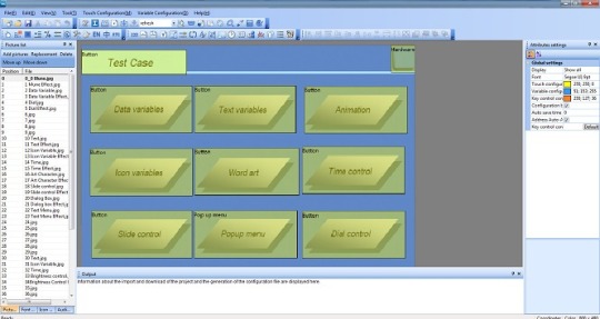
STONE TOOLBox软件
First, STONE is easy to use.With the STONE STONE TOOLBox software, you can easily create intuitive touch user interfaces, even if you're a beginner.
For example, by adding a static image as a background and defining functionality by component, you can easily and quickly create a simple GUI in just a few minutes.
With drag-and-drop components and simple instructions, you don't have to spend a lot of time on HMI project development.
Cost-effective
Engineers can easily develop the tft-lcd color user interface and touch control features, which can reduce a lot of development time and cost
The products are divided into three series, the advanced series for medical beauty, the industrial series for industrial electronics, and the lowest price for civil use.According to their own needs, choose the right type of screen.
Varieties
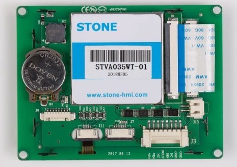
STONE HMI触摸屏
Various TFT LCD touch screen sizes from 3.5 inches, 4.3 inches, 5 inches, 5.6 inches, 5.7 inches, 7 inches, 8 inches, 10.1 inches, 10.4 inches, 12.1 inches, 15.1 inches, there are many models and options for the same size. With so many HMI displays, you are sure to find the best display for microcontroller projects like STM, RAM, Arduino and Raspberry Pi.。
STONE Support
Need help or technical help with your HMI project?Don't worry, STONE can provide technical support.
Optional UART interface type (RS232/RS485/TTL)
Optional touch control type (resistive/capacitive/non-touch)
STONE HMI Display
Industrial Type
Size Model Brightness Resolution View Area (mm) Voltage(V) Interface 3.5" STVI035WT-01 400 cd/m2 320x240 70.1x53.9 DC6.0-40 RS232/USB 4.3" STVI043WT-01 400 cd/m2 480x272 95x53.9 DC6.0-35 RS232/USB 5" STVI050WT-01 400 cd/m2 480x272 110.9x62.8 DC6.0-35 RS232/USB 5" STVI050WT-03 400 cd/m2 800x480 108x64.8 DC6.0-35 RS232/USB 5.6" STVI056WT-01 300 cd/m2 640x480 112.9x84.7 DC6.0-40 RS232/USB 7" STVI070WT-01 400 cd/m2 800x480 154.1x85.9 DC6.0-35 RS232/USB 7" STVI070WT-03 500 cd/m2 1024x600 154.1x85.9 DC6.0-35 RS232/USB 8" STVI080WT-01 400 cd/m2 800x600 162x121.5 DC6.0-40 RS232/USB 8" STVI080WT-03 400 cd/m2 1024x768 162x121.5 DC6.0-40 RS232/USB 10.1" STVI101WT-01 500 cd/m2 1024x600 222.7x125.3 DC6.0-40 RS232/USB 10.4" STVI104WT-01 350 cd/m2 800x600 211.2x158.4 DC6.0-40 RS232/USB
STONE HMI LCD module specifications:
Cortex m4 CPU; • UART interface (RS232/RS485/TTL) ; • 256-byte register; • 128 kb variable memory; • 128 MB flash memory, expandable to 1 GB; • GUI design software; • The customized command set; • 8-channel curve trend chart memory; • extremely fast variable display response speed; • The single-page supports up to 128 display variables; • Integrated real-time clock RTC, • Touch buzzer sound function; • Support software 90 degrees, 180 degrees, 270-degree screen rotation, adjust the appropriate visual Angle;
STONE TOOL Box (free GUI design software):
-- Free and easy to use STONE TOOL Box software
-- property value components that can be allocated at run time
-- Drag-and-drop components for GUI design and interaction
-- built-in debugger for HMI project emulation
STONE intelligent display module simple instructions:
UseTOOLS 2019 to design a GUI with any .jpg or .bmp image. 2. Use the UART interface (RS232/RS485/TTL) to communicate between the display and your MCU. 3. Use any language to write a simple program for the MCU, let it send the customized hex command sets to read or write the variable value of the display.
STONE LCD sample for developing:
For example: display the time variable "08: 30", and UART send the command: A5 5A 05 82 6F 00 08 30
Description:
A55A: Frame head 05: command byte length, 82 6F 00 08 30 total 5 bytes (excluding frame header) 82: write variable register command 6F 00: Variable address, set in control properties 08 30: data content, BCD code of 08 30
Package Including:
1 * STONE HMI 4.3" TFT 480x272 Resistive Lcd Touch Screen Intelligent Display Module
2 * Transfer board
2 * 8 pin terminal block
2 * 20mm long cable
1 * U disk
1 * USB cable
1 * 5mm short cable
1 * 20mm DB9 cable
STONE authentication and documentation:
- software
- editorial guide
- CE certification
- ROHS certification
- ISO9001 certification
- FC certification
STONE display starter
STONE consists of a hardware section (a series of TFT boards) and a software section (STONETOOL).
The STONE TFT board USES only one serial port for communication, thus avoiding wiring problems for users.
For the software part, STONE is rich in resources.
OSTONE - STONE TOOLBox is Windows software for GUI development.STONE TOOLBox has a number of components, such as buttons, text, progress bars, sliders, dashboards, and more, to enrich the interface design.In addition, drag-and-drop features reduce development effort by 99% by ensuring that users spend less time programming.With the help of this wysiwyg TOOLBox, designing guis becomes easy.
The STONE TOOLBox guide helps you easily set up the STONE TOOLBox.
O can communicate with STM, ARM, Arduino, Raspberry Pi.
The STONE TOOLBox guide helps you set up the STONETOOLBox software.
With these resources, I'm sure you'll have an easy experience on this monitor.
It is also easy to adapt the STONE series HMI to existing project users.You only need to provide one UART.
In addition, if you need any technical support when setting up the STONE display, you can contact STONE technical support.
STONE HMI Display Project idea
Here are some STONE HMI Display project ideas to get you started!
Use the STONE LCD module to create a refrigerator control
Reference: create refrigerator controls
Our fridge is not possible with any of the man-machine interface, but if there is a refrigerator with human-machine interface, let users can through the touch screen operation, control of refrigerator on the lower cooling efficiency, display the current the temperature inside the refrigerator, display the current indoor and outdoor temperature, and some feedback on the usage of refrigerator (days running, filter life, etc.), so, it is very convenient and practical for users.
What do you need?
Temperature sensor
Single chip microcomputer
STVC050WT-01for STM,ARM,Arduino Raspberry Pi general 5.0 inch HMI 480 * 272 touch display
Arduino IDEsoftware
STONE TOOLBoxsoftware
Running state includes:
Operation days
Filter element life
Outdoor temperature
Indoor temperature
To obtain these data, in addition to the first, the other three need the the corresponding sensor to collect these data. Filter element lifetime acquisition sensor and temperature sensor are required respectively. When the single-chip microcomputer collected these data, through the serial port to the designated display control address transmission data, the value of the display control on the corresponding change.
Running days can be implemented in two ways:
Use the RTC of STONE STVC050WT-01 serial port display screento display data directly on the screen
Use the single chip microcomputer's RTC to transfer data to the serial port screen for display
The STONE STVC050WT-01 serial port display comes with the RTC, which can be found in the STONE in development guide.
If you are interested, you can click: create refrigerator controlsSee the full tutorial!
STONE TFT LCD Module acceleration gyroscope sensor
With the STONE HMI display, you can now make an accelerometer gyroscope sensor. The accelerometer gyroscope sensor has the following functions:
Three text boxes display acceleration values
Three text boxes display the gyroscope values
Three text boxes display euler Angle values
A text box displays the current refresh time
Two buttons adjust the refresh time
What Do You Need
STONE advanced STVC070WT-01 universal 7-inch HMI touch screen
STM32F103RCT6 MCU
Mpu-6050 motion processing chip
Photoshop
Watch Dog
MPU-6050 Driver
Are you interested you can click Acceleration Gyroscope Sensor See the full tutorial!
Arduino uno + STONE LCD + Displays data read by MFRC522
reference:Displays data read by MFRC522
Due to my personal interest, I learned about the development of Arduino UNO and STONE LCD module project for two weeks, and found Arduino very simple, convenient and practical.So I wanted to do a simple demonstration with Arduino.I had an MFRC522 module at home, which I used in college, but I used STM32 to communicate with MFRC522, so I had to write my own driver for MFRC522 module, which was very complicated.
What Do You Need
STONE STVC050WT-01 display
Arduino UNO development board
MFRC522 module
Liquid crystal display
The MI card
Are you interested? You can go there https://www.stoneitech.com/news/sharing/how-to-display-data-read-by-mfrc522-through-stone-lcd-with-arduino.html Click to see the full tutorial!
LCD Arduino + STONE HMI +According to the heart rate
reference:instructables.com
Heart rate sensor module MAX30100 can collect users' blood oxygen and heart rate data, easy to use.
I found the MAX30100 library in the Arduino library file.That is, if you use communication between the LCD Arduino and the MAX30100, you can call the Arduino library file directly without having to rewrite the driver file.This is a good thing, so I bought the MAX30100 module.
I decided to use Arduino to verify the MAX30100's heart rate and oxygen collection capabilities.STONE TFT LCD screen for monitoring blood pressure.
What Do You Need
Arduino Mini Pro development board
MAX30100 heart rate and oxygen sensor module
STONE STVI070WT-01LCD serial display module
MAX3232 module
Are you interested you can click instructables.com See the full tutorial!
Conclusion
With STONE Display, you can now easily control and monitor STM, ARM, Arduino or Raspberry Pi machines, applications or device projects!Now, with the STONE STONE TOOLBox software, beginners can also create intuitive touch user interfaces.
What do you think of these STONE HMI displays?Let us know what you think of these STONE displays in the comments section below!
0 notes
Text
Trump may not be done with Jeff Sessions quite yet. Here's why
New Post has been published on https://newsprofixpro.com/tekamedia/2019/07/22/trump-may-not-be-done-with-jeff-sessions-quite-yet-heres-why/
Trump may not be done with Jeff Sessions quite yet. Here's why

Trump may not be done with Jeff Sessions quite yet. Here’s why
Read More
Buy Now


Price: $119.99
Item specifics
Condition: Used :
An item that has been used previously. The item may have some signs of cosmetic wear, but is fully operational and functions as intended. This item may be a floor model or store return that has been used. See the seller’s listing for full details and description of any imperfections. See all condition definitions– opens in a new window or tab
Seller Notes: “see description”
Brand:
Canon
Series: Canon EOS Digital Rebel Optical Zoom: 3x Type: Digital SLR Weight: 18 Oz. Connectivity: USB Color:
Black
Megapixels: 10.1MP Features: Auto Focus, Exposure Compensation Manufacturer Color: Black Custom Bundle: No MPN:
1236B001
Dimensions: H 3.7 X w 5.0 xD 2.6in. Screen Size: 2.5″ UPC:
0013803066098
About this product
Product Information Boost your photography skills and capture stunning photos with this Canon EOS Digital Rebel Digital SLR Camera. The Canon camera features 10.1-megapixel resolution, providing you with beautiful memories of your adventures. Perfect for taking pictures of objects at a distance, it is equipped with 3x optical zoom so that you can focus on images without sacrificing the resolution of your photos. A USB port is built into the camera, making it quick and easy to transfer your vacation pictures to your computer. Cherish every life event with this Canon EOS Digital Rebel Digital SLR Camera. Product Identifiers Brand Canon MPN 1236B001 UPC 0013803066098 Model XTi / EOS 400D eBay Product ID (ePID) 219530067 Product Key Features Optical Zoom 3x Color Black Features Auto Focus, Exposure Compensation Custom Bundle No Dimensions H 3.7 X w 5.0 xD 2.6in. Screen Size 2.5″ Series Canon EOS Digital Rebel Type Digital SLR Connectivity USB Megapixels 10.1MP Manufacturer Color Black Dimensions Weight 18 Oz. Additional Product Features Exterior Color Black Focal Length Range 1.6X Battery Type 2x Nb-2lh or 6X AA Batteries Sensor Resolution 10.1MP Camera Type Digital SLR Sensor Type Cmos Lens Aperture F/3.5-5.6 Battery Form Factor NB-2lh Lens for Sd EF-S 18-55mm Additional Features Exposure Compensation, Autofocus, USB Compatibility Display Size 2.5in.


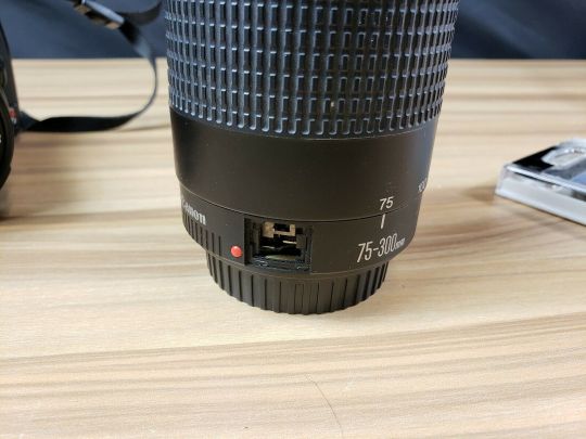


$119.99
End Date: Monday Aug-19-2019 11:24:10 PDT
Buy It Now for only: $119.99
Buy It Now | Add to watch list

Buy Now
Price: $114.95
Item specifics
Condition: Seller refurbished :
An item that has been restored to working order by the eBay seller or a third party not approved by the manufacturer. This means the item has been inspected, cleaned, and repaired to full working order and is in excellent condition. This item may or may not be in original packaging. See the seller’s listing for full details. See all condition definitions– opens in a new window or tab
Seller Notes: “Everything you see in the photos = EXCELLENT WORKING CONDITION – GUARANTEED!”
Brand:
Nintendo
MPN:
RR524765
Platform: Nintendo NES Model:
NES – Original
Country/Region of Manufacture: United States UPC:
0011152403427
About this product
Product Information You can go back in time to the roots of video games with the Nintendo Entertainment System Deluxe gray console. This classic Nintendo is a legend from the 1980s. This NES system can make gaming simple and fun for all ages. If you are looking for the perfect retro gift for your kids or someone young at heart, this system could be the perfect choice. You can let NES bring the original video game experience to your family. You can turn on the NES and let your kids enjoy “Super Mario Bros” for the first time. Mario and Luigi can jump right into their hearts. You can also introduce them to Mega Man, the legend that led to over 50 games spanning almost 30 years. You can watch their joy as they see Donkey Kong and his barrel bashing, or return to the roots of role-playing games with “Final Fantasy.” If you prefer traditional fighting games, you can try “Double Dragon.” You can test your survival skills with “Ice Climber.” You can reminisce about mall arcades with NES games like “Bubble Bobble” or “Tecmo Bowl.” These classic Nintendo games are only available on NES, which uses 8 bit graphics to depict your favorite characters completing goals or winning points. The system comes with 2 kB of RAM, which may be expanded with a console specific cartridge, as well as 256 bytes of OAM. The processing power of this console lets up to 64 sprites from your favorite game be displayed at once. Setting up your Nintendo console can be easy with no complicated accessories needed. You can connect your NES console to your television using a A/V or RCA cable. You can insert your game cartridge into the game slot, and start playing by following the prompts on your screen using the controller. The Nintendo controller has a simple look that complements the gray, black, and red system. The classic four arrow navigational panel lets you easily move through the game. The red “A” and “B” buttons are easy to use to control your character. Product Identifiers Brand Nintendo MPN RR524765 UPC 0011152403427 eBay Product ID (ePID) 101801921 Product Key Features Platform Nintendo NES Additional Product Features Product Name Nintendo Entertainment System Console Color Gray Type Console Product Line Nintendo Entertainment System Region Code NTSC Edition Deluxe

$114.95
End Date: Monday Jul-29-2019 17:41:43 PDT
Buy It Now for only: $114.95
Buy It Now | Add to watch list
0 notes
Last Seen Blogs

bitnxneun-blog
big boss x beauty


thirdpag
Third Pag

thebunnyandthefox2024
Bunny & Fox Adventures

inkren
Untitled