Last Seen Blogs


orangedodge
i'm not sure what goes here

funnyshit-blacknomadsoldier
!Funny Shit!

the-fault-in-our-cats-blog1
"Destiny Isn't A Path Any Cat Follows Blindly"

pillreminderapps-blog
Pill Reminder App | Best Medication Reminder App


Text
Oil
Millikan Oil Drop
Brenden Gerelle
Ben Luoma
December 7th, 2016
Abstract:
The aim of this experiment was to determine the charge of an electron experimentally. We did so by using a modified version of Millikan’s original Oil Drop Experiment. The most major of modifications would be no pressure chamber for our apparatus. We also used two methods for finding charged droplets, one being no starting voltage and spraying oil and the other being a starting voltage then spraying. The second method led us to question the variance in the mass of the oil droplets which was not found to be answered due to lack of trials. The electron charge we found was that of \( ( 2.13 \pm 0.10) \times 10^{-19} \space C \) [3] which is not within error of the established electron charge of \( (1.602 \pm 0.0000000098) \times 10^{-19} \space C \) [1]. Although we were not able to determine the known electron charge we were able to prove the quantization of electron charge. We found a \( +2 \) elementary charge to be \( 2.02 \pm 0.11 \) that of our \( +1 \) elementary charge.
Introduction:
After Thomas Rutherford discovered the existence of the electron in 1897, many people including Robert Millikan set out to determine the charge of the electron [3]. He did so by theorising with Harvey Fletcher about levitating charged oil droplets in the presence of an electric field. Since non-neutral oil droplets would experience a force proportional to the charge and electric field they set up an experiment to try and determine the electron charge. They succeeded in finding the elemetnary electron charge and determined it to within 1% of the established elementary charge value today. Their determined value was \( (1.5924 \pm 0.000017 ) \times 10^{-19} \space C \) [3] versus the verified value of experiment \( (1.602 \pm 0.0000000098 ) \times 10^{-19} \space C \) [1]. The experiment used in this report was based on Millikan’s experiment without the pressure chamber. The oil to be sprayed into the capacitor was that of paraffin oil and would gain or lose an electron due to friction of the tube of the atomizer or any other occurrence that would give an excess or lack of electrons. This effect enabled us to get charged oil droplets that would react to an electric field inside the capacitor. The experiment itself worked on the principle of a charge in an electric field producing a force parallel to that electric field as in the below equation.
\[ \boldsymbol{F} = q \boldsymbol{E} \]
Where \( \boldsymbol{F} \) is force
\( q \) is charge
\( \boldsymbol{E} \) is the electric field
The electric field would be produced by a capacitor with a DC power supply powering both plates with a potential difference. This in conjunction with a drag force and a force due to gravity produced a net force equilibrium as in figure 1.

Figure 1: Force equilibrium for a charge in an electric field against gravity [2]
It is important to note that buoyant force was ignored. Figure 1 leads to the net force equilibrium of
\[ q \boldsymbol{E} = m\boldsymbol{g} + k \boldsymbol{v_T} \]
Where \( m \) is mass in \( kg \)
\( \boldsymbol{g} \) is the acceleration due to gravity at the earth’s surface equal to \( 9.81 \frac{m}{s^2} \)
\( k \) is the drag coefficient
\( v_T \) is the terminal velocity of the oil droplet in \( \frac{m}{s} \)
Substituting
\[ V = - \int \boldsymbol{E} \cdot d \boldsymbol{l} \]
Where \( V \) is potential capable of \( 0 \) - \( 548 V \)
To get in terms of voltage and plate separation yields the force equilibrium equation. Since all directions are either up or down the vector notation was dropped.
\[ -q \frac{V}{l} = m g + k v_T \]
Where \( l \) is the plate separation distance equal to \( 0.005 \pm 0.0001 \space m \)
To express \( m \) in terms of something we can calculate we invokes Stokes’ Law to express mass as a simple density volume relationship with \(a\) being the radius of the droplet.
\[ a = \sqrt{\frac{9 \eta v_T}{2 g \rho}} \]
Where \( \eta \) is the viscosity of air equal to \( 1.84 \times 10^{-3} \space \frac{kg}{ms} \)
\( v_T \) is the terminal velocity in the presence of no electric field
\( \rho \) is the density of paraffin oil equal to \( 886 \space \frac{kg}{m^3} \)
It was noted that Stokes’ Law becomes invalid when the terminal velocity of the droplets is less than \( 0.1 \frac{cm}{s} \). This is due to the droplets having radii on the order of microns which are comparable to the mean free path of air molecules assumptions made in deriving Stokes’ Law. The velocities that will be seen in this experiment are on the order of \( 0.01 \) to \( 0.001 \space \frac{cm}{s} \) therefore the viscosity must be corrected by a factor of
\[ \eta_{eff} = \eta \frac{1}{1+\frac{b}{pa}} \]
Where \( b \) is a constant equal to \( 8.20 \times 10^{-3} \space Pa \cdot m \)
\( p \) is the standard barometric pressure in \( 101325 \space Pa \)
After substituting the equation above with the equation slightly higher (I have numbered equations in my word document so) we receive
\[ a=\sqrt{ \Big( \frac{b}{2p} \Big)^2 + \frac{ 9 \eta v_f}{2 g \rho }} - \frac{ b}{2p} \]
The sign ambiguity from the quadratic equation used in the derivation of the above equation was taken to be positive as radius is a positive quantity. The free fall velocity was determined from letting the without an electric field present as in Figure 2.

Figure 2: Force equilibrium for a falling spherical object [2]
With a radius, \(a\), we can now plug these substitutions back into the force equilibrium equation.
\[ -q \frac{V}{l} = \frac{4}{3} \pi a^3 \rho g + k v_T \]
Rearranging for \( v_T \) gives
\[ v_T = -\frac{4}{3} \frac{\pi a^3 \rho g}{k} - \frac{q}{lk}V \]
The equation above is in the form of a straight line which can be used to determine the drag coefficient, \( k \), and the charge, \( q \), with the help of a weighted linear ft of \( v_T \) versus \( V \).
\[ q =- w l k \]
Where \( w \) is the slope of the weighted linear fit
\[ k = - \frac{4}{3} \frac{\pi a^3 \rho g}{u} \]
Where \( u \) is the y-intercept of the weighted linear fit
Two methods were devised for spraying the oil into the capacitor. The first being, spray the oil with no voltage supplied to the capacitor plates, vary the potential difference to identify charged droplets, and then start recording their terminal velocities. The second method was to spray droplets into the capacitor with a nonzero potential difference across the plates. This allowed us to wait for uncharged droplets to drift off the viewing scope and leave only charged droplets that conformed to the electric field. This method begged the question as to whether or not there was enough variance in the oil droplet’s mass to get a multiple greater than 1 of the elementary electron charge. It should be noted that the potential difference across the plates manifests in an almost instantaneous electric field change as the time constant \( \frac{1}{RC} \) is very small. As well, the kinetic energy gained from the laser pointer used for allowing us to see our oil droplets was negligible and was ignored.
Procedure:
Our apparatus included a laser pointer, atomizer, viewing scope, capacitor, multiple stands, bubble level, electronic timer, paraffin oil, variable DC power supply, and a copper wire. The laser pointer was used to illuminate the inside of the capacitor so we could view the paraffin oil droplets through the viewing scope. The laser pointer was kept in its on orientation and propped up with a stand to keep the light in one place inside our capacitor. The capacitor was set on a stand and leveled with a bubble level to ensure our droplets fell vertically only. Using the copper wire, the viewing scope was focused to in range of the distance at which we would see the oil droplets. The viewing scope would then be finely focused for when oil droplets were inside the capacitor. We ran a few trials to verify we could see and control these charged droplets and to get a feel for how varying the voltage would vary the terminal velocity. Once we were ready, we sprayed oil into the capacitor with a starting voltage and varied while looking through the viewing scope to identify and control particles while the other person held the timer and recorded data. This strategy guaranteed more velocities recorded as one person could stop the droplet before it fell out while the other recorded the time dropping the chance that the droplet could fall off the viewing scope. The method of starting with a voltage difference across the plates guaranteed us to find a droplet that was slow enough to not fall out of the viewing scope and was used in the first 3 trials (Figure 5 as an example). All the remaining trials were done with the method of no starting voltage to enable us to get charges that were multiples that were greater than one of our elementary electric charge. Droplets that fell outside the grid before 9-10 recordings of velocities were disregarded as to get sufficient accurate data for our charge calculation. To record negative charges and/or charges with a high multiple of elementary charge we switched the two wires visible in Figure 3 to reverse the electric field direction and to control it more.

Figure 3: Picture of our experimental apparatus
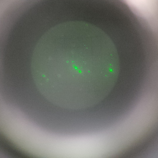
Figure 4: View through viewing scope with oil droplets inside the capacitor
Data:
To find terminal velocity from time we used a simple distance over time relationship where distance was one inner grid length, (Figure 5) which we took to be \( 0.0005 \space m\) [5], divided by time recorded on the electronic timer. Once we had the velocity we did a weighted linear fit to find both slope and y-intercept. We used the y-intercept value for \( v_T \) in the equation for radius of the oil droplet to find radius \(a \). With \( a\) known, we used the y-intercept again to solve for the drag coefficient \( k \) in the last equation. After \( k \) was found we took our weighted linear fit’s slope and used it in the second to last equation to solve for \(q\).

Figure 5: Starting Voltage of \( 275 \space V \)
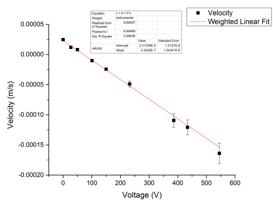
Figure 6: Starting voltage of \( 0 \space V \)
Figure 5 is an example of the +1 elementary charges we found. The no starting voltage method yielded charge values of,
\( (2.21 \pm 0.25) \times 10^{-19} \space C \)
\( (2.04 \pm 0.19) \times 10^{-19} \space C \)
\( (2.16 \pm 0.14) \times 10^{-19} \space C \)
As you can see with our method of starting with a potential difference we only obtained charge droplets with a single elementary charge.
Figure 6 was the only positive we recorded with a zero voltage and the value we received was,
\( (4.31 \pm 0.11) \times 10^{-19} \space C \)
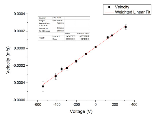
Figure 7: Starting voltage of \( 0 \space V \)
Figure 7 is an example of the negative charges we found. Two out of the three trials yielded a multiple of the elementary charge and the results to which can be found below
\( (-4.29 \pm 0.66) \times 10^{-19} \space C \)
\( (-2.25 \pm 0.08) \times 10^{-19} \space C \)
\( (-3.73 \pm 0.41) \times 10^{-19} \space C \)
To show quantization of charges we did a weighted average of the charges that we recorded more than one value of and took a simple ratio over lesser charges. The weighted average took the form,
\[ \overline{x} = \frac{ \sum_i \frac{x_i}{q_i^2}}{ \sum_i \frac{1}{q_i^2}} \]
\( +1 \) charge’s mean had a value of \( (2.13 \pm 0.10) \times 10^{-19} \space C \)
\( +2 \) charge’s mean had a value of \( (4.31 \pm 0.11) \times 10^{-19} \space C \)
\( -1 \) charge’s mean had a value of \( (-2.13 \pm 0.08) \times 10^{-19} \space C \)
\( -2 \) charge’s mean had a value of \( (-3.88 \pm 0.35) \times 10^{-19} \space C \)
Taking the ratios of the same sign charge yielded us,
\( +2 \) divided by \( +1 = 2.02 \pm 0.11 \)
\( -2 \) divided by \( -1 = 1.72 \pm 0.16 \)
Error
All error analysis will be done using standard error propagation (example given in the first two equations). Error in voltage was assumed to be negligible as it was electronic and would be smaller than our other errors. Time error was determined from multiple trials of trying to stop at 3 seconds then doing a histogram of the data and taking the standard deviation of the mean. Error in our distance for the velocity calculation was half of the smallest grid length (Figure 4). The weighted linear fit errors were determined from maple and examples of them can be found on the graphs. All constants are assumed to have zero error.
Our error values:
\( \Delta t = 0.08699 \space s\)
\( \Delta l = 0.0001 \space m\)
\( \Delta V \) ~ \( 0 \space V\)
\( \Delta d = 0.00005 \space m\)
\( \Delta u = \) error in y-intercept \( \frac{m}{s} \)
\( \Delta w = \) error in slope \( \frac{m}{sV} \)
\( \Delta v_T = \) error in terminal velocity
\( \Delta a = \) error in radius \( m\)
\( \Delta k = \) error in drag coefficient
\( \Delta q = \) error in charge in \( C \)
\( \Delta \overline{x} = \) error in weighted average in \( C \)
\( \Delta \frac{ q_2 }{q_1} = \) error in charge ratio
\[ \Delta v_T = \sqrt{ \Big( \frac{\partial v_T}{\partial d} \cdot \Delta d \Big)^2 + \Big( \frac{\partial v_T}{\partial t} \cdot \Delta t \Big)^2} \]
\[ \Delta v_T = \sqrt{ \Big( \frac{ \Delta d }{t} \Big)^2 + \Big( \frac{d \Delta t}{t^2} \Big)^2 } \]
\[ \Delta a = \frac{9 \eta \Delta v_T }{ 4 g \rho \sqrt{ \big( \frac{b}{2p} \big)^2 + \frac{9 \eta v_T}{2 g \rho} } }\]
\[ \Delta k = \sqrt{ \Big(\frac{4}{3} \frac{\pi a^3 p g \Delta u }{ u^2} \Big)^2 + \Big( \frac{4 \pi a^2 p g \Delta a}{ u } \Big)^2 } \]
\[ \Delta q = \sqrt{ ( \Delta l k w )^2 + ( l \Delta k w )^2 + ( l k \Delta w )^2 } \]
\[ \overline{x} = \frac{1}{\sum_i \frac{1}{\sigma_i^2}} \]
\[ \Delta \frac{ q_2 }{q_1} = \sqrt{ \Big( \frac{q_2 \Delta q_1}{q_1^2} \Big)^2 + \Big( \frac{\Delta q_2}{q_1} \Big)^2} \]
Conclusion:
Although our calculated elementary charge \( (2.13 \pm 0.10) \times 10^{-19} C \) was not within the standard value of \( (1.602 \pm 0.0000000098) \times 10^{-19} \) we were able to prove the quantized nature of charge. Taking the mean of our \( +2 \) charge then dividing it by our \( +1\) charge gave us a ratio of \( 2.02 \pm 0.11 \) which is well within error of the \( +2 \) charge being a multiple of \( +1 \) by an integer number. The \( -2 \) charge mean divided by the \( -1 \) charge was \( 1.72 \pm 0.16 \) which is not within error of an integer multiple. This is mostly due to lack of trials for the negative charges to gain sufficient lack of error for an accurate result. As well we didn’t collect sufficient data to extrapolate on the variance of the mass in our droplets that would yield a higher elementary charge than \( 1 \). Our charges were always higher than the standard value implying there was a systematic error within our experiment. One cause could not be using a pressure chamber. Other reasons include getting the exact value for the grid length in our viewing scope (assumed to be \( 0.5 \space mm \)) [5] and using the y-intercept for finding both the drag coefficient \( k \) and the radius \( a \). It was realised too late that the calculation was done using the y-intercept and could not be rectified. Improvements to this lab would be using a pressure chamber to encapsulate your capacitor, Using the recorded free fall velocity to calculate \( a \) instead of the y-intercept, and refining our time error by recording a droplet falling multiple times and taking the standard deviation of the plotted histogram
References
[1] "CODATA Value: Elementary Charge". Physics.nist.gov. N.p., 2016. Web. 7 Dec. 2016.
[2] "Millikan Oil-Drop Experiment | Electrostatics". Kshitij-iitjee.com. N.p., 2016. Web. 7 Dec. 2016.
[3] "Millikan's Oil Drop Experiment (Theory) : Modern Physics Virtual Lab : Physical Sciences : Amrita Vishwa Vidyapeetham Virtual Lab". Vlab.amrita.edu. N.p., 2016. Web. 7 Dec. 2016.
[4] "Robert Millikan". Aps.org. N.p., 2016. Web. 7 Dec. 2016.
[5] Instruction Manual And Experiment Guide For The PASCO Scientific Model AP-8210. 1st ed. Roseville: Pasco, 2016. Web. 7 Dec. 2016.
0 notes
Text
working on something
\[ E=mc^2\]
\[ E=mc^2\]
\[ E=mc^2\]
\[ E=mc^2\]
\[ E=mc^2\]
\[ E=mc^2\]
\[ E=mc^2\]
\[ E=mc^2\]
\[ E=mc^2\]
\[ E=mc^2\]
\[ E=mc^2\]
\[ E=mc^2\]
\[ E=mc^2\]
\[ E=mc^2\]
\[ E=mc^2\]
\[ E=mc^2\]
\[ E=mc^2\]
\[ E=mc^2\]
\[ E=mc^2\]
\[ E=mc^2\]
\[ E=mc^2\]
\[ E=mc^2\]
\[ E=mc^2\]
\[ E=mc^2\]
\[ E=mc^2\]
\[ E=mc^2\]
\[ E=mc^2\]
\[ E=mc^2\]
\[ E=mc^2\]
\[ E=mc^2\]
\[ E=mc^2\]
\[ E=mc^2\]
\[ E=mc^2\]
\[ E=mc^2\]
\[ E=mc^2\]
\[ E=mc^2\]
\[ E=mc^2\]
\[ E=mc^2\]
\[ E=mc^2\]
\[ E=mc^2\]
\[ E=mc^2\]
\[ E=mc^2\]
\[ E=mc^2\]
\[ E=mc^2\]
\[ E=mc^2\]
\[ E=mc^2\]
\[ E=mc^2\]
\[ E=mc^2\]
\[ E=mc^2\]
\[ E=mc^2\]
\[ E=mc^2\]
\[ E=mc^2\]
\[ E=mc^2\]
\[ E=mc^2\]
\[ E=mc^2\]
\[ E=mc^2\]
\[ E=mc^2\]
\[ E=mc^2\]
\[ E=mc^2\]
\[ E=mc^2\]
\[ E=mc^2\]
\[ E=mc^2\]
\[ E=mc^2\]
\[ E=mc^2\]
\[ E=mc^2\]
\[ E=mc^2\]
\[ E=mc^2\]
\[ E=mc^2\]
\[ E=mc^2\]
\[ E=mc^2\]
\[ E=mc^2\]
\[ E=mc^2\]
\[ E=mc^2\]
\[ E=mc^2\]
\[ E=mc^2\]
\[ E=mc^2\]
\[ E=mc^2\]
\[ E=mc^2\]
\[ E=mc^2\]
\[ E=mc^2\]
\[ E=mc^2\]
\[ E=mc^2\]
\[ E=mc^2\]
\[ E=mc^2\]
\[ E=mc^2\]
\[ E=mc^2\]
\[ E=mc^2\]
\[ E=mc^2\]
\[ E=mc^2\]
\[ E=mc^2\]
\[ E=mc^2\]
\[ E=mc^2\]
\[ E=mc^2\]
\[ E=mc^2\]
\[ E=mc^2\]
\[ E=mc^2\]
\[ E=mc^2\]
\[ E=mc^2\]
\[ E=mc^2\]
\[ E=mc^2\]
\[ E=mc^2\]
\[ E=mc^2\]
\[ E=mc^2\]
\[ E=mc^2\]
\[ E=mc^2\]
\[ E=mc^2\]
\[ E=mc^2\]
\[ E=mc^2\]
\[ E=mc^2\]
\[ E=mc^2\]
\[ E=mc^2\]
\[ E=mc^2\]
\[ E=mc^2\]
\[ E=mc^2\]
\[ E=mc^2\]
\[ E=mc^2\]
\[ E=mc^2\]
\[ E=mc^2\]
\[ E=mc^2\]
\[ E=mc^2\]
\[ E=mc^2\]
\[ E=mc^2\]
\[ E=mc^2\]
\[ E=mc^2\]
\[ E=mc^2\]
\[ E=mc^2\]
\[ E=mc^2\]
\[ E=mc^2\]
\[ E=mc^2\]
\[ E=mc^2\]
\[ E=mc^2\]
\[ E=mc^2\]
\[ E=mc^2\]
\[ E=mc^2\]
\[ E=mc^2\]
\[ E=mc^2\]
\[ E=mc^2\]
\[ E=mc^2\]
\[ E=mc^2\]
\[ E=mc^2\]
\[ E=mc^2\]
\[ E=mc^2\]
\[ E=mc^2\]
\[ E=mc^2\]
\[ E=mc^2\]
\[ E=mc^2\]
\[ E=mc^2\]
\[ E=mc^2\]
\[ E=mc^2\]
\[ E=mc^2\]
\[ E=mc^2\]
\[ E=mc^2\]
\[ E=mc^2\]
\[ E=mc^2\]
\[ E=mc^2\]
\[ E=mc^2\]
\[ E=mc^2\]
\[ E=mc^2\]
\[ E=mc^2\]
\[ E=mc^2\]
\[ E=mc^2\]
\[ E=mc^2\]
\[ E=mc^2\]
\[ E=mc^2\]
\[ E=mc^2\]
\[ E=mc^2\]
\[ E=mc^2\]
\[ E=mc^2\]
\[ E=mc^2\]
\[ E=mc^2\]
\[ E=mc^2\]
\[ E=mc^2\]
\[ E=mc^2\]
0 notes
Text
Suppose we had a wire. In this wire there are positive charges moving along the wire to the right with speed \( v \). Assume the charges are close enough together such that we can treat them as a continuous line charge \( \lambda \). Likewise there’s a flow of electrons with continuous line charge \( - \lambda \) moving to the left at the same speed \( v \). Since we have negative charges moving there’s a current \( I \) with magnitude
\[ I = 2 \lambda v \]
Suppose we were to put an charged particle \( q \) a distance \( s \) away from the wire moving at speed \( u < v \). Because we have both a stream of charges going to the left and right in the wire of equal magnitude they cancel off leaving electrical force on the charged particle. The demonstration of the above can be seen in the top wire below which we will call \( S \)
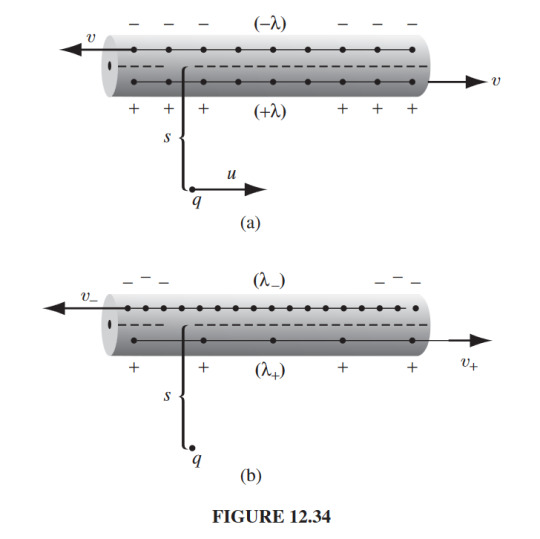
Now consider the frame of the particle in which the particle \( q \) is at rest (bottom picture). We will call this frame \( \overline{S} \). Since our particle is now at rest in the frame the positive charges are now further and further apart and the negative line charge is now more densely packed together
0 notes
Text
coffeeve sleeve
I made quite a few mistakes computing these PDEs but i’m going to leave them up just because plz ignore :)
errors that I’m able to point out right now without looking are cosine being \( (-1)^n \) instead of \( 1 \), constant calculation is wrong, and other egregious errors but I took my PDE class 4 years ago ish so
A good learning resource for analytical PDEs
https://ocw.mit.edu/courses/mathematics/18-303-linear-partial-differential-equations-fall-2006/lecture-notes/heateqni.pdf
0 notes
Text
Proper time is invariant under Lorentz Transformations
\( ds^2 = c^2 dt^2 - dx^2 - dy^2 - dz^2 \)
under an \(x\) direction boost such that
\( t’ = \gamma ( t - \frac{vx}{c^2} ) \)
\( x’ = \gamma (x-vt) \)
\( y’ = y \)
\( z’ = z \)
With \( \gamma = \frac{1}{\sqrt{1-\frac{v^2}{c^2}}} \)
Taking the infinitesimals
\( dt’ = \gamma (dt - \frac{v}{c^2} dx) \)
\( dx’ = \gamma (dx-v dt) \)
\( dy’ = dy \)
\( dz’ = dz \)
Proper time under the boost
\( ds’^2 = c^2 dt’^2 - dx’^2 - dy’^2 - dz’^2 \)
\( ds’^2 = c^2 \gamma^2 (dt - \frac{v}{c^2} dx)^2 - \gamma^2 (dx-v dt)^2 - dy^2 - dz^2 \)
\( ds’^2 = c^2 \gamma^2 (dt^2 - 2 \frac{v}{c^2} dx dt + \frac{v^2}{c^4} dx^2) - \gamma^2 (dx^2 -2v dx dt + v^2 dt^2) - dy^2 - dz^2 \)
\( ds’^2 = c^2 \gamma^2 dt^2 -2 \gamma^2v dx dt + \gamma^2 \frac{v^2}{c^2} dx^2 - \gamma^2 dx^2 + 2 \gamma^2 v dx dt - \gamma^2 v^2 dt^2 - dy^2 - dz^2 \)
\( ds’^2 = c^2 \gamma^2 dt^2 - \gamma^2 v^2 dt^2 -2 \gamma^2v dx dt + 2 \gamma^2 v dx dt + \gamma^2 \frac{v^2}{c^2} dx^2 - \gamma^2 dx^2 - dy^2 - dz^2 \)
\( ds’^2 = \gamma^2 (c^2-v^2) dt^2 + \gamma^2 (\frac{v^2}{c^2} - 1) dx^2 - dy^2 - dz^2 \)
\( ds’^2 = \gamma^2 (1 - \frac{v^2}{c^2} ) c^2 dt^2 - \gamma^2 (1 -\frac{v^2}{c^2}) dx^2 - dy^2 - dz^2 \)
Remember \( \gamma = \frac{1}{\sqrt{1-\frac{v^2}{c^2}}} \)
\( ds’^2 = \frac{1}{1-\frac{v^2}{c^2}}(1 - \frac{v^2}{c^2} ) c^2 dt^2 - \frac{1}{1-\frac{v^2}{c^2}} (1 -\frac{v^2}{c^2}) dx^2 - dy^2 - dz^2 \)
\( ds’^2 =c^2 dt^2 - dx^2 - dy^2 - dz^2 \)
\( ds’^2 =ds^2 \)
0 notes
Text
The Schrodinger equation in three spatial dimensions
\( i \hbar \frac{\partial }{\partial t} \Psi = \Big[ - \frac{\hbar^2}{2m} \nabla^2 + V(x,t) \Big] \Psi \)
Follows the same pattern except time is imaginary compared to the spatial components
0 notes
Text
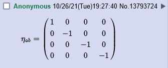
Time is a psuedo dimension
\( \eta_{00} = 1,\space \eta_{11} = -1, \space \eta_{22} = -1, \space \eta_{33} = -1, \space \eta_{i \neq k} = 0 \)
or
\[
$\begin{pmatrix}
1 & 0 & 0 & 0\
0 & -1 & 0 & 0\
0 & 0 & -1 & 0\
0 & 0 & 0 & -1 \end{pmatrix}$
\]
\( \begin{matrix}
1 & 2 & 3\ \
a & b & c
\end{matrix} \)
\( \begin{matrix}
1 & 2 & 3\ \
a & b & c
\end{matrix} \)
\(
\begin{matrix}
1 & 2 & 3\\
a & b & c\\
3 & 4 & 54
\end{matrix}\)
\(
\begin{smallmatrix}
1 & 2 & 3\\
a & b & c\\
3 & 4 & 54
\end{smallmatrix}\)
\( \begin{smallmatrix} 1 & 2 \\ 3 & 4 \end{smallmatrix} \)
\begin{pmatrix} 1 & 2 & 3\\ a & b & c\\ 3 & 4 & 54 \end{pmatrix}
\eta_{ab} =
\begin{smallmatrix}
1 & 0 & 0 & 0\\
0 & -1 & 0 & 0\\
0 & 0 & -1 & 0\\
0 & 0 & 0 & -1\\
\end{smallmatrix}

0 notes
Text
wtf is this
\( \nabla \cdot E = \frac{\rho}{\epsilon_0} \)
\( \epsilon_0 = \frac{1}{c^2 \mu_0} \)
\( \nabla \cdot E = \rho c^2 \mu_0 \)
Assume even distribution of charge throughout volume
\( \rho = \frac{q}{V} \)
\( \nabla \cdot E = \frac{q}{V} c^2 \mu_0 \)
\( \frac{V}{ \mu_0 } \nabla \cdot E = q c^2 \)
Dimensional analysis
\( m^3 m^{-1} kg^{-1} s^2 A^2 kg s^{-3} A^{-1} = C m^2 s^{-2} \)
\( m^2 s^{-1} A = C m^2 s^{-2} \)
\( m^2 s^{-1} A = m^2 s^{-1} C s^{-1} \)
Assuming current is constant
\( A = \frac{C}{s} \)
\( m^2 s^{-1} A = m^2 s^{-1} A \)
Huh
Electronvolts
Why am I even thinking about this
Because charge is always indicative of mass so you can equate the two
\( q \propto m \)
\( \frac{V}{ \mu_0 } \nabla \cdot E = q c^2 \)
\( \frac{V}{ \mu_0 } \nabla \cdot E \propto m c^2 \)
Does this look familiar?
11:07 pm 21/11/01
With calculus (I chose to choose linearity because looks better)
\( \int_V \nabla \cdot E dV= \int_V \rho c^2 \mu_0 dV \)
\( \int_V \nabla \cdot E dV= q c^2 \mu_0 \)
\( \frac{1}{ \mu_0 } \int_V \nabla \cdot E dV= q c^2 \)
\( \frac{1}{ \mu_0 } \int_V \nabla \cdot E dV \propto m c^2 \)
0 notes
Text
fight me
https://brundungerelle.tumblr.com/post/117329874388
0 notes
Text
Taking a break
This shit is tedious as fuck and the only reason I took such a long break is because of that. Emphatically fuck PDEs, numerical solutions exist for a raisin
0 notes
Text
Consider a coffee that is completely insulated at both ends
Mathematically this takes for the form
\( \frac{\partial}{\partial x} T(0,t) = \frac{\partial}{\partial x} T(h,t) =0 \)
With the initial condition that the top fifth of the coffee is cooled to freezing point
\( T(x,0) = T_1, 0 \leq x \leq 0.8h\) and \( T_2, 0.8h < x \leq h\)
We can apply separation of variables because we have homogeneous boundary conditions and do so
\( \frac{\partial}{\partial t}T(x,t) = \frac{\partial^2}{\partial x^2} T(x,t) \)
\( T(x,t) = \beta \chi(x) \tau(t) \)
\( \frac{\partial}{\partial t} \chi(x) \tau(t) = \beta \frac{\partial^2}{\partial x^2} \chi(x) \tau(t) \)
\( \chi(x) \tau’(t) = \beta \chi’’(x) \tau(t) \)
\( \frac{1}{ \beta } \frac{\tau’(t)}{ \tau(t)} = \frac{\chi’’(x)}{ \chi(x) } \)
We see that both derivatives are equal to eachother even though they differ by differentiation variable so they must be equal to a constant such that
\( \frac{1}{ \beta } \frac{\tau’(t)}{ \tau(t)} = \frac{\chi’’(x)}{ \chi(x) } = -\lambda \)
Separate into two ODEs (wow!)
\( \frac{1}{ \beta } \frac{\tau’(t)}{ \tau(t)} = -\lambda \)
\( \frac{1}{ \beta } \frac{\tau’(t)}{ \tau(t)} +\lambda =0 \)
\( \frac{1}{ \beta } \tau’(t) +\lambda \tau(t) =0 \)
\( \frac{\chi’’(x)}{ \chi(x) } = -\lambda \)
\( \frac{\chi’’(x)}{ \chi(x) } + \lambda =0 \)
\( \chi’’(x) + \lambda \chi(x) =0 \)
Which now has the form of two individual ordinary differential equations
Assume the solution takes the form of a wave in exponential form \( e^{rx} \)
\( \chi’’(x) + \lambda chi(x) =0 \)
\( r^2e^{rx} + \lambda e^{rx} =0 \)
Dividing off the exponential. If you allow the imaginary r to exist then you can see dividing this off in both forms of a wave is valid (another way to look at the \( \lambda \) equivalency)
\( r^2 + \lambda =0 \)
\( r^2 = - \lambda \)
\( r = \sqrt{- \lambda } \)
So \( r \) depends on 3 cases which consist of
\( \lambda <0 \), \( \lambda = 0 \), and \( \lambda > 0 \)
Supoose \( \lambda <0 \):
\( r = \sqrt{- -\lambda} = \sqrt{ \lambda} \)
which says \( \lambda \) is positive so we assume the solution takes the form
\( \chi(x) = c_1 cosh( \sqrt{ \lambda} \ x) + c_2 sinh( \sqrt{ \lambda} x) \)
Using boundary conditions to determine constants
\( \frac{\partial}{\partial x} T(0,t) = \frac{\partial}{\partial x} T(h,t) =0 \)
\( chi’(x) = c_1 \sqrt{\lambda} sinh(\sqrt{\lambda} x) + c_2 \sqrt{\lambda} cosh{\sqrt{\lambda} x}) \)
\( chi’(0) = c_1 \sqrt{\lambda} sinh(\sqrt{\lambda} 0) + c_2 \sqrt{\lambda} cosh(\sqrt{-lambda} 0) = 0 \)
\( chi’(0) = c_2 \sqrt{\lambda} cosh(\sqrt{\lambda} 0) = 0 \)
\( chi’(0) = c_2 \sqrt{\lambda} = 0 \)
Since we want nontrivial eigenvalues we take \( c_2 = 0 \)
\( chi’(x) = c_1 \sqrt{\lambda} sinh(\sqrt{\lambda} x) \)
Second boundary condition
\( chi’(0) = c_1 \sqrt{\lambda} sinh(\sqrt{\lambda} h) = 0 \)
Since \( sinh( x ) \) is only zero at the vertical axis thus we require \( c_1 = 0 \)
Second case \( \lambda = 0 \):
\( \chi’’(x) + \lambda chi(x) =0 \)
\( \chi’‘(x) = 0 \)
Integrating twice
\( \chi(x) = c_1 x + c_2 \)
\( \chi(0) = 0 \)
\( \chi(x) = c_1 0 + c_2 = 0 \)
\( c_2 = 0 \)
\( \chi(h) = 0 \)
\( \chi(h) = c_1 h = 0 \)
We assume \( h \neq 0 \) thus
\( c_1 = 0 \)
Again we get the trivial solution where \( chi(x) = 0 \)
Case 3 \( \lambda > 0 \):
\( r = \sqrt{- \lambda } \)
\( r = i\sqrt{ \lambda } \)
???????????????????????????? clarify
We have an imaginary exponential as the root(s) to \( r \)
\( \therefore \) the solution takes the form (can you guess with euler’s formula?)
\( \chi(x) = c_1cos \big( \sqrt{ \lambda } x \big)+c_2 sin \big( \sqrt{ \lambda } x \big) \)
\( \chi’(x) = \frac{\partial}{\partial x} c_1cos \big( \sqrt{ \lambda } x \big)+ \frac{\partial}{\partial x} c_2 sin \big( \sqrt{ \lambda } x \big) \)
\( \chi’(x) = \sqrt{ \lambda } \frac{\partial}{\partial x} c_2 cos \big( \sqrt{ \lambda } x \big) - \sqrt{ \lambda } c_1sin \big( \sqrt{ \lambda } x \big) \)
\( \chi’(0) = \sqrt{ \lambda } c_2 cos \big( \sqrt{ \lambda } (0) \big) - \sqrt{\lambda } c_1 sin \big( \sqrt{ \lambda} (0) \big) = 0 \)
\( \chi’(0) = \sqrt{ \lambda } c_2 cos \big( \sqrt{ \lambda } (0) \big) - \sqrt{\lambda } c_1 sin \big( \sqrt{ \lambda} (0) \big) = 0 \)
\( \chi’(0) = \sqrt{ \lambda } c_2 = 0 \)
Non trivial eigenvalues
\( c_2 = 0 \)
\( \chi’(h) = - \sqrt{\lambda } c_1 sin \big( \sqrt{ \lambda} (h) \big) = 0 \)
If we set \( \sqrt{\lambda} = \frac{ n \pi}{h} \) then we get zeroes regardless of \( c_1 \) \( \therefore \) we have the non trivial solution to \( \chi (x) \)
\( \chi(x) = c_n cos \big( \frac{ n \pi}{h} x \big) \)
for \( 0 \leq x \leq h \)
Now for the time ODE
\( \frac{1}{ \beta } \tau’(t) +\lambda \tau(t) =0 \)
we know \( \lambda > 0 \) thus
\( \frac{1}{ \beta } \tau’(t) = - \lambda \tau(t) \)
\( \tau’(t) = - \beta \lambda \tau(t) \)
We notice this takes the form \( \frac{ d}{dx} e^{-\beta \lambda x} = -\beta \lambda e^{-\beta \lambda x} \) Therefore
\( \tau(t) = C e^{-\beta \lambda t} \)
Plugging in our value for \( \lambda \)
\( \tau(t) = C_n e^{-\beta \big( \frac{n \pi}{h} \big)^2 t} \)
Combining our two seperate ODEs into one PDE
\( T(x,t) = \beta \chi(x) \tau(t) \)
\( T(x,t) = c_n cos \big( \frac{ n \pi}{h} x \big) C_n e^{-\beta \big( \frac{n \pi}{h} \big)^2 t} \)
Combining constants
\( T(x,t) = c_n cos \big( \frac{ n \pi}{h} x \big) e^{-\beta \big( \frac{n \pi}{h} \big)^2 t} \)
We use the initial condition
\( T(x,0) = f(x) \)
\( T(x,0) = c_n cos \big( \frac{ n \pi}{h} x \big) e^{-\beta \big( \frac{n \pi}{h} \big)^2 (0)} \)
we can see the exponential term goes to zero therefore we’re left with
\( T(x,0) = c_n cos \big( \frac{ n \pi}{h} x \big) \)
to determine what \( c_n \) is by integrating
\( c_n = \int_0^h f(x) cos \big( \frac{ n \pi}{h} x \big) dx \)
we set \( T(x,0) = f(x) = T_1, 0 \leq x \leq 0.8h\) and \( T_2, 0.8h < x \leq h \)
HOLY FUCK
0 notes
Text
Consider a coffee that is completely insulated at both ends such that
\( \frac{\partial}{\partial x} T(0,t) = \frac{\partial}{\partial x} T(h,t) =0 \)
With the initial condition that the top fifth of the coffee is cooled to freezing point
\( T(x,0) = T_1, 0 \leq x \leq 0.8h\) and \( T_2, 0.8h < x \leq h\)
We apply separation of variables
0 notes
Text
Mother fucker
I just realized I made the substitution for \( cos(n pi) \) to be \( 1 \) instead of \( (-1)^n \)
Disgraceful
FUCK
Have to redo that shit anyway
0 notes
Text
I don’t like the fixed temperature endpoints approximation so I insulate both ends
Also changing my initial heat distribution to be the top one fifth of the coffee being cooled due to the ice instantly melting it to that temperature

I can’t really get the approximation to be that accurate but roughly looking at the pattern you can see the temperature difference between two initial temperatures is different

0 notes