ok-x - Tumblr blog

ok-x · 4 years

Text

Week 4

import pandas as pd import numpy import seaborn import matplotlib.pyplot as plt data = pd .read_csv('gapminder.csv',low_memory=False)

sub2grp = sub2.groupby('incomeperperson')

#find average for each income level print("average values for each income level") mean = sub2grp.mean() print(mean)

# change format from numeric to categorical sub2["incomperperson"]=sub2["incomeperperson"].astype('category')

seaborn.countplot(x="incomeperperson",data=sub2); plt.xlabel('Income per person') plt.title('2010 Gross Domestic Product per capita')

seaborn.distplot(sub2["incomeperperson"].dropna(),kde=False); plt.xlabel('Income per person') plt.title('2010 Gross Domestic Product per capita')

seaborn.distplot(sub2["alcconsumption"].dropna(),kde=False); plt.xlabel('Alcohol consumption') plt.title('2008 alcohol consumption per adult (age 15+), litres')

sub2["suicideper100th"]=["suicideper100th"].astype('category') seaborn.distplot(sub2=["suicideper100th"].dropna(),kde=False); plt.xlabel('Suicide rate') plt.title('Mortality due to self-inflicted injury, per 100 000 standard population') c2=sub2.groupby('alcconsumption').size()

#association charts scat1=seaborn.regplot(x="incomeperperson",y="alcconsumption",data=sub2) plt.xlabel('Income per person') plt.ylabel('Alcohol consumption') plt.title('Scatterplot for the Association between income per person and alcohol consumption')

scat2=seaborn.regplot(x="incomeperperson",y="suicideper100th",data=sub2) plt.xlabel('Income per person') plt.ylabel('Suicide rate') plt.title('Scatterplot for the Association between income per person and suicide rate')

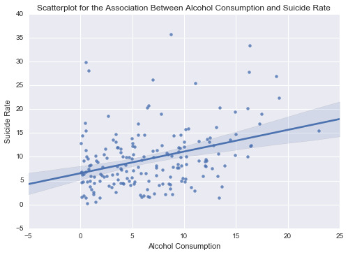
scat3=seabron.regplot(x="alcconsumption",y="suicideper100th") plt.xlabel('Alcohol consumption') plt.ylabel('Suicide rate') plt.title('Scatterplot for the Association between alcohol consumption and suicide rate')

Here are the histograms for the variables:

The first one is the histogram for the variable ‘Alcohol consumption’. It has a unimodal distribution, the mode is between 0 and 2.5 litros of alcohol consumpted in a year.

The second chart is the histogram for the variable ‘Suicide’. The graph has a unimodal distribution as well, the mode is approximately between 7.5 and 10 in the suicide rate.

The third chart is the histogram for the variable ‘Income per Peson’. It has a unimodal distribution as well, the distribution seem like a exponetial curve.

THE ASSOCIATION:

The scatterplot between the alcohol consumption and the suicide rate show positive association, meaning that those countries with higher values in the alcohol consumption rate have higher values in the suicide rate.

0 notes

ok-x · 4 years

Text

Week 3

My Data Management Decision

import pandas as pd import numpy data = pd .read_csv('gapminder.csv',low_memory=False)

data['alcconsumption'] = pd.to_numeric(data['alcconsumption'],errors="coerce") data['suicideper100th'] = pd.to_numeric(data['suicideper100th'],errors="coerce") data['incomeperperson'] = pd.to_numeric(data['incomeperperson'],errors="coerce")

print("counts for income per person") c1 = data["incomeperperson"].value_counts(sort=False) print(c1) print("percentages for income per person") p1= data["incomeperperson"].value_counts(sort=False,normalize=True) print(p1) print("counts for alcohol consumption") c2=data ["alcconsumption"].value_counts(sort=False) print(c2) print("percentages for alcohol consumption") p2=data["alcconsumption"].value_counts(sort=False,normalize=True) print(p2) print("counts for suicide rate per 100k ") c3=data["suicideper100th"].value_counts(sort=False) print(c3) print("percentages for suicide rate per 100k") p3=data["suicideper100th"].value_counts(sort=False,normalize=True) print(p3)

#subset data to include only country, income, alcohol consumption rate and suicide rate

sub1 = data[['country','incomeperperson','alcconsumption','suicideper100th']] sub2=sub1.copy()

sub2['incomeperperson'] = sub2['incomeperperson'].replace(' ' ,numpy.nan) sub2['alcconsumption'] = sub2['alcconsumption'].replace(' ' ,numpy.nan) sub2['suicideper100th'] = sub2['suicideper100th'].replace(' ' ,numpy.nan) #drop any rows that have NaN for any cell sub2 = sub2.dropna()

ds1= sub2['incomeperperson'].describe() print(ds1)

#split data into 4 groups by income sub2['incomeperperson'] = pd.cut(sub2['incomeperperson'],[0,2000,5000,10000,60000],labels=["very low","low","medium","high"]) #counts and percentages for each income level print("counts for income per person") ct = sub2['incomeperperson'].value_counts(sort=False,dropna=False) print(ct)

print("percentages for income per person") pt = sub2['incomeperperson'].value_counts(sort=False,dropna=False,normalize=True) print(pt)

#group data by income per person sub2grp = sub2.groupby('incomeperperson')

#find average for each income level print("average values for each income level") mean = sub2grp.mean() print(mean)

The output

Name: incomeperperson, dtype: float64 counts for income per person very low 79 low 32 medium 27 high 39 Name: incomeperperson, dtype: int64 percentages for income per person very low 0.446328 low 0.180791 medium 0.152542 high 0.220339 Name: incomeperperson, dtype: float64

counts for income per person very low 79 low 32 medium 27 high 39

average values for each income level

incomeperperson alcconsumption suicideper100th

very low 4.690633 9.758873 low 7.453438 9.672904 medium 9.092222 10.028339 high 9.144872 9.046834

0 notes

ok-x · 4 years

Text

Week 2

1) My program:

import pandas import numpy data = pandas.read_csv('gapminder.csv',low_memory=False) data.columns = map(str.upper, data.columns)

pandas.set_option('display.float_format',lambda x:'%f'%x)

print(len(data)) print(len(data.columns))

data['incomeperperson']=data['incomeperperson'].convert_objects(convert_numeric=True) data['alcconsumption']=data['alcconsumption'].convert_objects(convert_numeric=True) data['suicideper100th']=data['suicideper100th'].convert_objects(convert_numeric=True)

#subset data to include only country, income, alcohol consumption rate and suicide rate

sub1 = data[['country','incomeperperson','alcconsumption','suicideper100th']]

2)The output:

213 16

The Gapminder dataset consists 213 observations or rows and 16 variables or columns.

Counts for income per person column

Counts for alcohol consumption

Counts for suicide rate per 100k

0 notes

ok-x · 4 years

Text

Week 1

1) After looking through the codebook for the Gapminder dataset, I have decided that I am interested in discovering the situation of alcohol consumption all around the world. 2) There are many different things that affect the rate of alcohol consumption and they vary from country to country. Specifically, I would like to analyze the association between alcohol consumption per adult and income per person. Afterward, I am interested to also explore whether there is a connection between alcohol consumption rate and suicide rate across the world.

I have included these 3 variables in my personal codebook for further analysis.

3) On the first topic about the association between alcohol consumption and income rate I found a few types of research conclusions of which are quite controversial. Findings have indicated that people with higher socioeconomic status may consume similar or greater amounts of alcohol compared with people with lower socioeconomic status. Also, they mentioned that people who did not graduate from high school and had a low income had the lowest prevalence of heavy episodic drinking. At the same time, another research made in the USA claims that Higher rates of past heavy alcohol use or alcohol abuse/dependence were found among the unemployed people.

So, according to the studies I read, I can make a hypothesis that the connection between alcohol consumption and income rate undoubtedly exists. Nevertheless, this rate varies by many other variables such as general socioeconomic status, country of residence, access to alcohol.

4) On the second topic about the association between alcohol consumption and suicide rate the researches, I found that the scholars agreed in principle on the same conclusion. According to the one research, The association between alcohol consumption and suicide rates have been analyzed in 13 nations of the world, where 10 in 10/13, suicide rates were positively associated with per capita consumption of alcohol. In three nations, this relationship was not found. The inconsistent results of epidemiological studies of the relation between alcohol use and suicide indicate that multiple sociocultural and environmental factors influence suicide rates and that studies conducted in one nation are not always applicable to other nations. Another study proves this hypothesis by claiming that there is no direct link between alcohol dependence and suicide rates. It is all connected in one system which includes socio-cultural factors, the mental state of a person, and etc. Suicide is committed by people as a result of mental problems that could be caused by alcohol addiction.

Literature review:

Associations Between Socioeconomic Factors and Alcohol Outcomes. Susan E. Collins, Ph.D.

A systematic review of the influence of the community level social factors on alcohol use. Bryden A, Roberts B, Petticrew M, McKee M.

Interactive Influences of Neighborhood and Individual Socioeconomic Status on Alcohol Consumption and Problems. Nina Mulia, Katherine J. Karriker-Jaffe

Time series analysis of alcohol consumption and suicide mortality in the United States, 1934-1987.Journal of Studies on Alcohol, 59(4), 455–461 (1998).

Alcohol consumption and suicide . L. Sher

1 note · View note