naduahcoursera

[naduahcoursera]

K-Means Cluster Analysis

Program

proc surveyselect data=clust out=traintest seed = 123 samprate=0.7 method=srs outall; run;   data clus_train; set traintest; if selected=1; run; data clus_test; set traintest; if selected=0; run; * standardize the clustering variables to have a mean of 0 and standard deviation of 1; proc standard data=clus_train out=clustvar mean=0 std=1; var h1gi20 ethnicity h1to11 h1to30 h1gh1 h1pr4 h1ed7 h1ed5 h1gi11 h1nb5 drinking bio_sex; run; %macro kmean(K); proc fastclus data=clustvar out=outdata&K. outstat=cluststat&K. maxclusters= &K. maxiter=300; var h1gi20 ethnicity h1to11 h1to30 h1gh1 h1pr4 h1ed7 h1ed5 h1gi11 h1nb5 drinking bio_sex; run; %mend; %kmean(1); %kmean(2); %kmean(3); %kmean(4); %kmean(5); %kmean(6); %kmean(7); %kmean(8); %kmean(9); * extract r-square values from each cluster solution and then merge them to plot elbow curve; data clus1; set cluststat1; nclust=1; if _type_='RSQ'; keep nclust over_all; run; data clus2; set cluststat2; nclust=2; if _type_='RSQ'; keep nclust over_all; run; data clus3; set cluststat3; nclust=3; if _type_='RSQ'; keep nclust over_all; run; data clus4; set cluststat4; nclust=4; if _type_='RSQ'; keep nclust over_all; run; data clus5; set cluststat5; nclust=5; if _type_='RSQ'; keep nclust over_all; run; data clus6; set cluststat6; nclust=6; if _type_='RSQ'; keep nclust over_all; run; data clus7; set cluststat7; nclust=7; if _type_='RSQ'; keep nclust over_all; run; data clus8; set cluststat8; nclust=8; if _type_='RSQ'; keep nclust over_all; run; data clus9; set cluststat9; nclust=9; if _type_='RSQ'; keep nclust over_all; run; data clusrsquare; set clus1 clus2 clus3 clus4 clus5 clus6 clus7 clus8 clus9; run; * plot elbow curve using r-square values; symbol1 color=blue interpol=join; proc gplot data=clusrsquare; plot over_all*nclust; run; ***************************************************************************************** further examine cluster solution for the number of clusters suggested by the elbow curve ***************************************************************************************** * plot clusters for 4 cluster solution; proc candisc data=outdata4 out=clustcan; class cluster; var h1gi20 ethnicity h1to11 h1to30 h1gh1 h1pr4 h1ed7 h1ed5 h1gi11 h1nb5 drinking bio_sex; run; proc sgplot data=clustcan; scatter y=can2 x=can1 / group=cluster; run; * validate clusters on GPA; * first merge clustering variable and assignment data with GPA data; data clust; set clus_train; keep id_num h1to2; run; proc sort data=outdata4; by id_num; run; proc sort data=clust; by id_num; run; data merged; merge outdata4 clust; by id_num; run; proc sort data=merged; by cluster; run; proc means data=merged; var h1to2; by cluster; run; proc anova data=merged; class cluster; model h1to2 = cluster; means cluster/tukey; run;

Output

Summary

A k-means cluster analysis was conducted to identify underlying subgroups of adolescents based on their similarity on 11 variables that could have an impact on age of first smoking. Clustering variables included seven binary categorical variables measuring whether adolescents had ever tried drinking, cannabis, or snuff/chewing tobacco, whether they felt their neighbourhood was safe or unsafe, if they had ever been held back in school, if they had been suspended and if they were born in the US as well as biological sex. Clustering variables also included a 6-category ethnicity variable, a 5-scale friend support variable, a their grade in school, a self-rated measure of health on a 5-point scale. All clustering variables were standardized to have a mean of 0 and a standard deviation of 1.

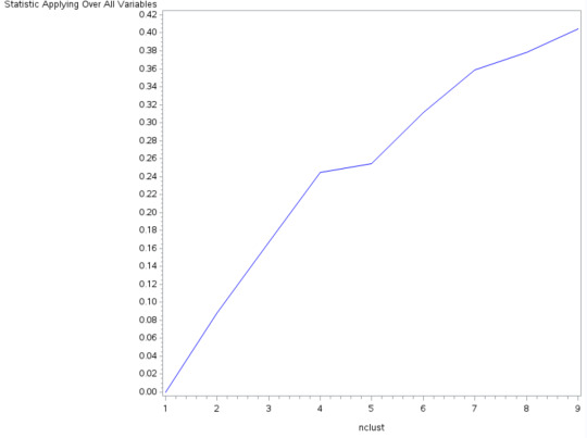
Data were randomly split into a training set that contained 70% of the data (n=4553) and a test set that contained 30% of the observations (n=1900). A series of k-means cluster analyses were conducted on the training data specifying k=1-9 clusters, using Euclidean distance. The variance in the clustering variables that was accounted for by the clusters (r-square) was plotted for each of the nine cluster solutions in an elbow curve seen above to provide guidance for choosing the number of clusters. The elbow curve was inconclusive, but suggested 4 might be a good cut off. Following is an interpretation of the 4-cluster solution.

Canonical discriminant analyses were used to reduce the variables down to the variables that accounted for the most variance in the clustering variables. A scatterplot can be seen above of the first two canonical variables by cluster. The four clusters are tightly packed and distinct, which suggested low within cluster variance and high variance between clusters, which supports the interpretation of 4-cluster solution.

The means on the cluster variables suggested that youth in cluster 1 were slightly whiter or mixed, had moderate snuff use, were much more likely to have used cannabis, had the best health, had moderate friend support, were moderately likely to have been held back or suspended, and were the least likely to drink. Cluster 2 were the second oldest group, more white than cluster 1, the least likely to have used snuff or chewing tobacco, had moderate health, had the lowest friend support, were the most likely to have been suspended or held back, but lived in the safest neighbourhoods. Cluster 3 were the oldest group and the most ethnically diverse. They also had the second highest snuff/chewing tobacco use, the least cannabis use, the second poorest health, and the most likely to drink. The fourth cluster were the youngest, had the highest snuff use, the poorest health, the most friend support, were the least likely to have been held back a grade, the most likely to be born in the US, and the second most likely to drink. Overall, the biggest differences between clusters seemed to be along grade and ethnicity lines.

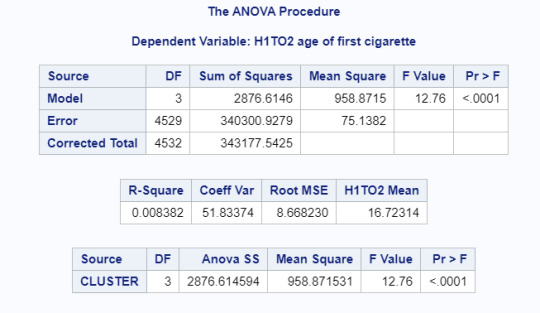
In order to externally validate the clusters, an Analysis of Variance (ANOVA) was conducted to test for significant differences between the clusters on age of first cigarette. A tukey test was used for post hoc comparisons between the clusters. Results indicated significant differences between the clusters on first age of smoking (F(3, 4529)=12.76, p<.0001). Tukey post hoc comparisons showed significant differences between clusters on smoking between all groups except clusters 1 and 3. Youth in cluster 2 had the lowest age of first smoke (mean=14.557, sd=6.48) and youth in cluster 1 had the highest age of first smoke (mean=19.955, sd=6.78). 

Limitations of this include that there are many binary categorical variables in this analysis and that there are significant differences between the clusters and how groups are distributed.

[naduahcoursera]

Lasso Regression Analysis

Selected Code

proc surveyselect data=new out=traintest seed=1325 samprate=0.7 method=srs outall; run; proc glmselect data=traintest plots=all seed=1325; /*lasso regression with LAR algorithm and k=10*/ partition ROLE=selected(train='1' test='0'); model h1pr4=drinking smoking white highschool h1nb5 h1gi11 health h1ed5 bio_sex h1ed7 snuff cannabis/selection=lar (choose=cv stop=none) cvmethod=random(10);

Select Output

Summary

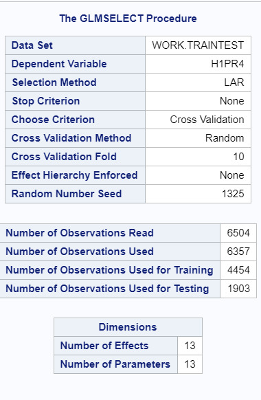
A lasso regression analysis was conducted to identify a subset of variables from a pool of 12 categorical explanatory variables that best predicted a quantitative response variable measuring friend support in adolescents. Ethnicity was measured in a binary categorical variable comparing white and non-white adolescents. Binary substance use variables were used based on questions on if youth had ever tried drinking, smoking, or chewing tobacco/snuff. Additional categorical variables included: grade level, sorted into a binary categorical variable for high school or middle school; neighbourhood safety (H1NB5) which was a binary measure of if youth felt safe in their neighbourhoods; immigrant status (H1GI11), a binary categorical variable based on if a youth was born in the US or not; health, which was binned into a binary categorical variable of “good” and “poor” health; grade retention, that is, whether a youth had been held back in a grade (H1ED5), biological sex, and whether the youth had ever been suspended (H1ED7). All predictor variables were standardized to have a mean of zero and a standard deviation of one.

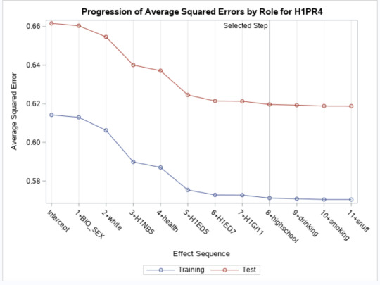
Data were randomly split into a training set that included 70% of the observations (N=4454) and a test set with the remaining 30% of the observations (N=1903). The least angle regression algorithm with a k=10 cross fold validation test was used to estimate the lasso regression model in the training set and the model was validated using the test set. The change in the mean squared error at each step was used to identify the best subset of predictor variables.

Of the 12 predictor variables, 9 were retained in the selected model. During the estimation process, sex, ethnicity, neighbourhood safety, and health were most strongly associated with friend support as seen in Coefficient Progression. Other predictors associated with friend support included grade retention, suspension history, immigrant status and grade level. However, these variables only accounted for 7% of the variance in the friend support response variable as seen in the R-Square. 

[naduahcoursera]

Random Forests

Code

proc hpforest; target smoking/level=nominal; input drinking friendsupport white highschool h1nb5 h1gi11 health h1ed5 h1ed7 snuff cannabis/level=nominal; run;

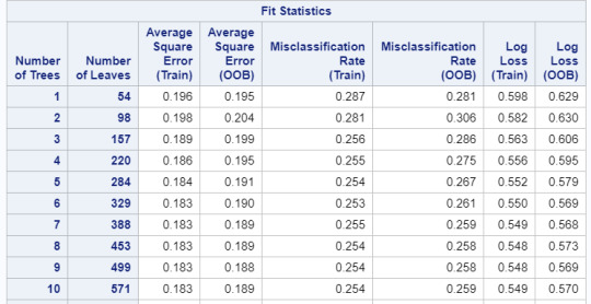
Error Rate

First and Last 10 Trees

Importance

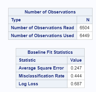
Random forest analysis was performed to evaluate the potential importance of a series of explanatory variables in predicting a binary, categorical response variable. In this case, the response variable was if youth had tried smoking. Potential explanatory variables included were: drinking (if youth had tried drinking or not), if youth had ever been suspended (H1ED7), grade level (high school or not), ethnicity (white or non-white), chewing tobacco/snuff use, self-rated health (poor or good), cannabis use, immigrant status (H1GI11) meaning if a youth had been born in the US or not, grade retention/if a youth had been held back (H1ED5), neighbourhood safety (H1NB5), and self-reported support by friends.

Drinking, by far, had the highest relative importance. Suspension, grade level, ethnicity, and snuff use were all also considered important. The accuracy of the model was 66% overall. Within the model, Error Rate was similar between the training and OOB models and suggests further interpretation of a single tree may be appropriate and accurate for the rest of the sample.

[naduahcoursera]

Classification Tree

Program

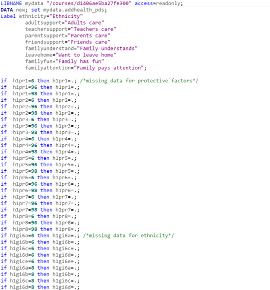
LIBNAME mydata "/courses/d1406ae5ba27fe300" access=readonly; DATA new; set mydata.addhealth_pds; label ethnicity="Ethnicity" friendsupport="Friends care" H1pr4="Friend Support" h1nb5="Neighborhood Safety" h1gi20="School Grade" h1to2="First Time Smoking" H1TO14="First Time Drinking" h1nb5="Neighborhood Safety";

if h1to2=96 then h1to2=.; /*missing data for cigarettes*/ if h1to2=97 then h1to2=.; /*legitimate skip*/ if h1to2=98 then h1to2=.; if h1to2=0 then h1to2=.; /*never smoked whole cigarette*/ if H1TO14=96 then H1TO14=.; /*refused*/ if H1TO14=97 then H1TO14=.; /*never drank or not with parents*/ if H1TO14=98 then H1TO14=.; /*don't know*/ if h1pr1=6 then h1pr1=.; /*missing data for protective factors*/ if h1pr1=96 then h1pr1=.; if h1pr1=98 then h1pr1=.; if h1pr3=6 then h1pr3=.; if h1pr3=96 then h1pr3=.; if h1pr3=98 then h1pr3=.; if h1pr4=6 then h1pr4=.; if h1pr4=96 then h1pr4=.; if h1pr4=98 then h1pr4=.; if h1gi6a=6 then h1gi6a=.; /*missing data for ethnicity*/ if h1gi6b=6 then h1gi6b=.; if h1gi6c=6 then h1gi6c=.; if h1gi6d=6 then h1gi6d=.; if h1gice=6 then h1gi6e=.; if h1gi6a=8 then h1gi6a=.; if h1gi6b=8 then h1gi6b=.; if h1gi6c=8 then h1gi6c=.; if h1gi6d=8 then h1gi6d=.; if h1nb5=6 then h1nb5=.; if h1nb5=8 then h1nb5=.; if h1gi20=96 then h1gi20=.; if h1gi20=97 then h1gi20=.; if h1gi20=98 then h1gi20=.; if h1gi20=99 then h1gi20=.;

/*Data Management*/ numethnic=sum (of h1gi4 h1gi6a h1gi6b h1gi6c h1gi6d); if numethnic GE 2 then ethnicity=1; /*multiple race and ethnic groups*/ else if h1gi4=1 then ethnicity=3; /*Latinx or Hispanic*/ else if h1gi6b=1 then ethnicity=2; /*Black or African American*/ else if h1gi6a=1 then ethnicity =0; /*White*/ else if h1gi6c=1 then ethnicity=4; /*Native*/ else if h1gi6d=1 then ethnicity=5; /*Asian or Pacific Islander*/

if h1gi20 ge 9 then highschool=1; else if h1gi20 < 9 then highschool=0;

if h1pr4 GE 4 then friendsupport=1; /*high friend support*/ else friendsupport=2; /*low friend support*/

if h1to2>=13 then smoking=2; /*average age or higher*/ else smoking=1;

if h1to14>=15 then drinking=2; /*research shows lower risk*/ else drinking=1;

if ethnicity=0 then white=1; else white=0; if ethnicity=0 then Black=0; else if ethnicity=2 then Black=1; if ethnicity=0 then Latinx=0; else if ethnicity=3 then Latinx=1; if ethnicity=0 then Native=0; else if ethnicity=4 then Native=1; if ethnicity=0 then Asian=0; else if ethnicity=5 then Asian=1; if ethnicity=1 then mixedwhite=1; else if ethnicity=0 then mixedwhite=0; if ethnicity=1 then mixedblack=1; else if ethnicity=2 then mixedblack=0; proc sort; by AID; ods graphics on; proc hpsplit seed=42992; class smoking drinking friendsupport white highschool h1nb5; model smoking= drinking friendsupport white highschool h1nb5; grow entropy; prune costcomplexity; RUN;

Clasification Tree

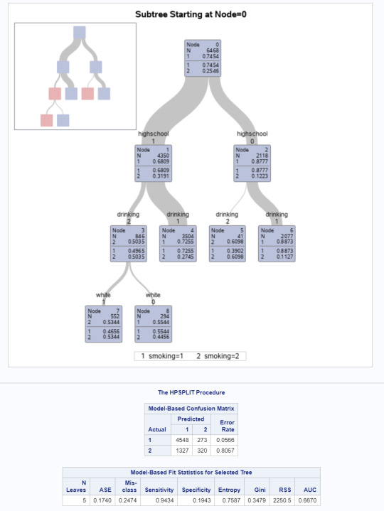
Classification tree analysis was performed to test nonlinear relationships among a series of explanatory variables and a binary, categorical response variable (high risk first age of smoking). Entropy “goodness of split” criterion was used to grow the tree and the cost-complexity algorithm was used for pruning into the final tree.

Explanatory variables used were: ethnicity(white/non-white), high risk drinking (beginning before age 15), grade level (high school or middle school), and neighbourhood safety. These were used to analyse the target variable: age of first smoking (separated above and below average, 13 years of age). This sample removed those who have not had a full drink or cigarette as missing data.

Grade level was the first variable to separate the sample into subgroups. In youth in high school (n=4350, range 9-12), 68% of youth began smoking before 13 compared to 87% of those in middle school. Further subdivisions were made for age of first drink. High schoolers who had drunk before age 15 (considered high risk by NIAA) were more likely to smoke before age 13 (73%) compared to those who had a drink after age 15 (50%). Middle schoolers who drank before age 15 were far more likely to have smoked before age 13 (89% vs. 39%). The final subdivision was for youth in high school who had their first drink after age 15, which was divided into white and non-white. Non-white, low-risk drinking, high school students were less likely to smoke before age 13 (47% vs 55%). 

The total model was better at predicting high-risk first-time smokers than non-smokers. The model classified 75% of the sample overall and was better at predicting high-risk smokers than low-risk smokers. The model correctly predicted 94% of high-risk first-time smokers (Sensitivity) and only 19% of low-risk smokers (Specificity). 

#Continue adding variables #Add in non-smokers and non-drinkers

[naduahcoursera]

Logistic Regression

My research question was examining the relationship between ethnicity and friend support in the ADDHealth study. In this logistic regression, I also controlled for grade (binned into a binary categorical value of “high school=1” for grades 9-12 and “high school=0″ for grades 7-8, and neighbourhood safety where 0=unsafe and 1=safe.

After adjusting for confounding factors (grade level and neighbourhood safety), the odds of feeling high support from friends were about two times higher for white youth than for non-white youth (OR=2.058, CI=1.79-2.365, p<.0001), which supports my hypothesis. Neighbourhood safety (H1NB5) was also significantly associated where youth in safe neighbourhoods were about two times more likely to feel high friend support than those in unsafe neighbourhoods (OR=2.163, CI=1.796-2.606, p<.0001). Grade level was not significantly associated with youth friend support. 

There was not evidence of confounding as the individual variables were significant and positive before and after controlling for other variables. Individually, ethnicity showed that white youth were 2.239 times more likely to report friend support (CI=1.954=2.585, p<.0001) and neighbourhood safety showed that youth in safe neighbourhoods were 2.5 times more likely to report friend support (CI=2.085-3.004, p<.0001). 

[naduahcoursera]

Multiple Regression

My research question has been examining if there is an association between ethnicity and how supported youth feel by friends. For this analysis, I decided to also add neighbourhood safety (if youth feel safe or unsafe in their neighbourhood) and grade level as possible confounding variables. For simplicity, I collapsed the ethnicity variable into “white” and “POC” to make it a binary categorical variable where white=1, non-white=0. For the purposes of this assignment, friend support (a variable with a response scale) is considered quantitative. Neighbourhood safety (H1NB5) is a binary categorical variable with unsafe=0 and safe=1. I centered grade level because there is no 0 age.

My hypothesis is that there is an association between ethnicity and friend support.

Linear Regression (no confounders)

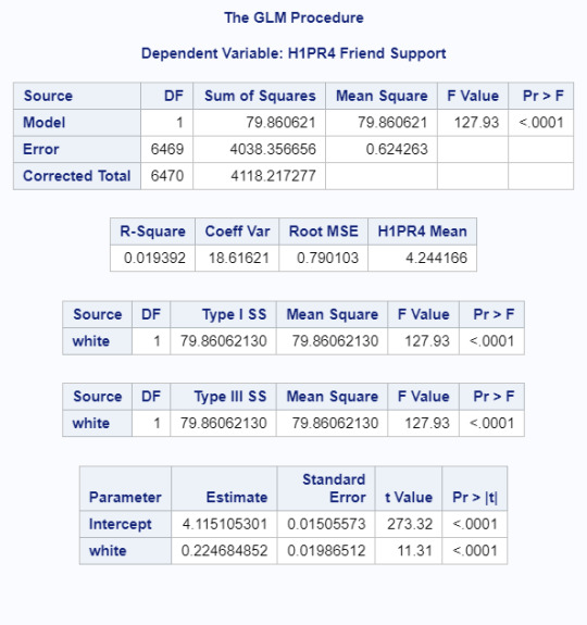
The initial regression showed a significant (Beta=0.22, p<.0001) positive relationship between ethnicity and how supported youth felt by friends. The line of best fit equation was Friend Support = 4.115+(white)*.22. What this actually means is that the mean response for non-white youth was 4.115 and the mean response for non-white students was 4.335. That said, the r^2 is very low (.019) meaning this only explains 2% of the variability in friend support responses.

Multiple Regression

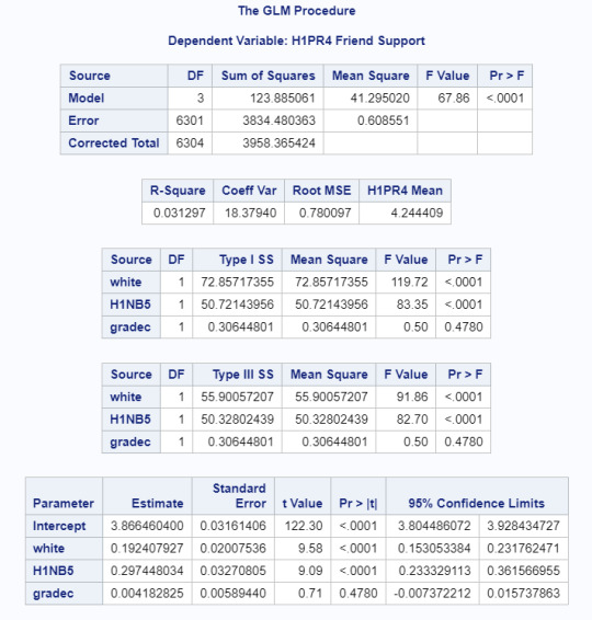
After adjusting for potential confounders (neighbourhood safety and grade level), ethnicity (Beta=0.192, p<.0001) was significantly and positively associated with friend support. Neighborhood safety was also significantly associated with friend support where youth in safe neighbourhoods were more likely to feel supported (Beta=0.297, p<.0001) than those in unsafe neighbourhoods. Grade level was not significantly associated with friend support. There is not evidence of confounding because the relationship remained true even with added variables. Again, the R-Square is very low (.03) meaning this only explains 3% of the variability in friend support responses, which is further supported by the regression diagnostic plots below.

Regression Diagnostic Plots

The Q-Q plot assumes standard distribution and the residuals should follow a line. Here, it’s clear that the residuals for friend support do not follow expected standard distribution. Given the linear groupings, it seems likely that part of this is because for the purposes of this assignment, we are treating this as a quantitative variable rather than a categorical variable. 

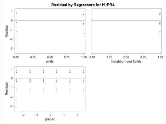
The standard residuals plot tests how many residuals fall within one standard deviation of the mean. Normal distribution would assume that 95% of residuals should fall within 1 standard deviation of the mean. Here it is clear, that is not the case. While 95% of residuals fall within 1 standard deviation above, many are as far away as 3 standard deviations away. This is more than 5% having an absolute value greater than or equal to 2.5 and that means the standard of error for this model would be considered unacceptable and this model does not properly fit what is occurring.

Finally, the leverage and outlier plot examines what outliers may be influencing the data, how likely they are to be influencing model fit, and any values that have significant leverage to change the predict scores for other observations. While there are a lot of outliers and possible leverage points in this data, they are all incredibly close to 0, which implies that these do not have significant power to affect the regression model. That means that despite the many outliers and leverage points and the poor fit of the model, these outliers and leverage points are not where the errors in the model lie.

[naduahcoursera]

Linear Regression

My research question is investigating how ethnicity and protective factors are associated, specifically how ethnicity and how supported by friends youth are.

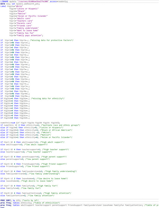
Program

LIBNAME mydata "/courses/d1406ae5ba27fe300" access=readonly; DATA new; set mydata.addhealth_pds; Label ethnicity="Ethnicity" H1pr4="Friend Support";

/*missing data for protective factors*/ if h1pr4=6 then h1pr4=.; if h1pr4=96 then h1pr4=.; if h1pr4=98 then h1pr4=.; if h1gi6a=6 then h1gi6a=.; /*missing data for ethnicity*/ if h1gi6b=6 then h1gi6b=.; if h1gi6c=6 then h1gi6c=.; if h1gi6d=6 then h1gi6d=.; if h1gice=6 then h1gi6e=.; if h1gi6a=8 then h1gi6a=.; if h1gi6b=8 then h1gi6b=.; if h1gi6c=8 then h1gi6c=.; if h1gi6d=8 then h1gi6d=.;

/*Data Management*/ numethnic=sum (of h1gi4 h1gi6a h1gi6b h1gi6c h1gi6d); if numethnic GE 2 then ethnicity=1; /*multiple race and ethnic groups*/ else if h1gi4=1 then ethnicity=4; /*Latinx or Hispanic*/ else if h1gi6b=1 then ethnicity=3; /*Black or African American*/ else if h1gi6a=1 then ethnicity =2; /*White*/ else if h1gi6c=1 then ethnicity=5; /*Native*/ else if h1gi6d=1 then ethnicity=6; /*Asian or Pacific Islander*/

if ethnicity=2 then white=0; else white=1;

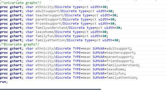
PROC SORT; by AID; /*sorts by id*/ proc freq; tables ethnicity; /*table of ethnicities*/ proc freq; tables friendsupport; /*table of protective factor*/ /*univariate graphs*/ proc gchart; vbar ethnicity/Discrete type=pct width=15; proc gchart; vbar friendsupport/Discrete type=pct width=15;

/*Bivariate graphs*/ proc gchart; vbar ethnicity/discrete TYPE=mean SUMVAR=friendsupport;

proc freq; tables friendsupport*ethnicity/chisq;

proc freq; tables white h1pr4; proc glm; model h1pr4=white;

Frequency Table

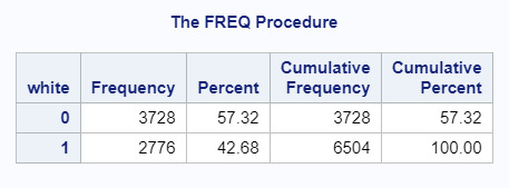
Centered frequency table for ethnicity collapsed into two-category variable (white=0, POC=1).

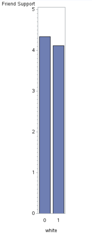
Regression

The results of the linear regression indicated that ethnicity (Beta=-.22, p<.0001) was significantly and negatively associated with support from friends. What this equation (Response Variable=4.34+(Explanatory*-.22)) means is that rather than a line of best fit, white participants will have an average response of 4.34 and non-white participants will have an average response of 4.1 as confirmed with the bivariate graph below.

[naduahcoursera]

Writing About Data

Sample

The sample is from the first wave of the National Longitudinal Study of Adolescent to Adult Health (Add Health). This study followed a nationally representative sample of U.S. participants from adolescence through adulthood. Wave one was completed during the 1994-1995 school year, surveying 7-12th graders. Level of analysis is at the individual level with 90,000 adolescents surveyed. My specific data set, focusing on ethnicity and protective factors has fewer participants (n=6423). Of those participants, 10% were mixed race (n=683), 58% were white (n=3728), 23% were Black (n=1468), 5% were Latinx (n=326), .6% were Native (40), and 3% were Asian (n=208).

Procedure

Data was collected through school-based surveys and in-home interviews during the 1994-1995 school year. All students on a school roster were eligible to be surveyed. The in-school survey measured social and demographic information and in-home interviews measured health status, nutrition, decision-making, family composition, romantic relationships, and more. For each adolescent, one parent, usually the mother, also completed an interviewer-assisted questionnaire.

Measures

Ethnicity was measured in a series of questions that comprehensively captured ethnic information. Hispanic or Latino origin was asked first and if youth answered yes, further information about specific ancestral history was asked, otherwise youth skipped to the next series of ethnicity questions. For each ethnicity asked (white, Black or African American, Native American or American Indian, and Asian or Pacific Islander), youth were able to mark or not mark their response, refuse, or mark “I don’t know”. Protective factors (specifically, adults caring, parents caring, and friends caring) were all asked in a similar manner. For each variable, youth were asked “How much do you feel that adults/parents/your friends care about you?” and marked their answer on a 5-point scale (1-Not at all, 2-Very little, 3-Somewhat, 4-Quite a bit, 5-Very much) along with options for “Does Not Apply”, “Refused”, and “Don’t Know”. 

To manage my data, I created a new variable for ethnicity, that could collapse the five different ethnicity questions into one variable. This variable first identified any participant who marked more than one ethnicity and categorized them as mixed race, which ensured their other responses were not double counted in further analysis. After separating mixed race participants, each yes response for each individual ethnicity was coded as its own response for the new ethnicity variable. To make analysis of response variables easier, the three protective factor variables were each binned into two-category variables. Missing values were removed, then each protective factor was sorted into “high” or “low” caring, with the new “high category” including 4 and 5 responses from the original scale, and the “low” category including 1, 2, and 3 responses. 

[naduahcoursera]

Chi-Square with Moderator

Syntax

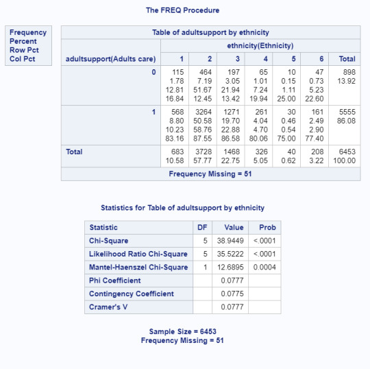
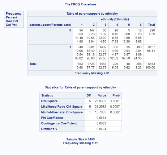
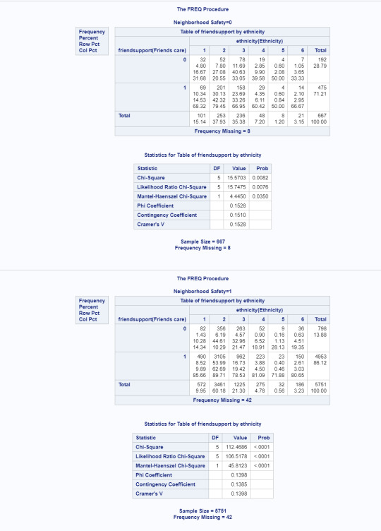
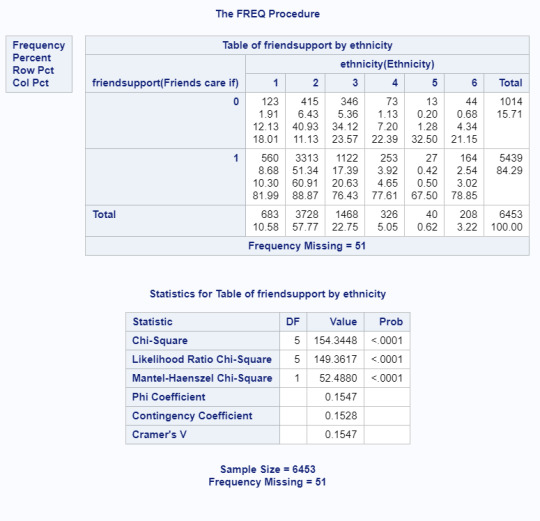
proc sort; by h1nb5; proc freq; tables adultsupport*ethnicity/chisq; by h1nb5; proc freq; tables parentsupport*ethnicity/chisq; by h1nb5; proc freq; tables friendsupport*ethnicity/chisq; by h1nb5;

Chi-Square Output

My research question is examining how ethnicity is associated with protective factors (specifically adult support, parent support and friend support) in the ADDHealth study. To see my initial Chi-Square results, you can click here.  Here I’ve decided to investigate how neighbourhood safety may be a moderating factor. I’ve included select output charts for my results because the actual number of tables is too numerous due to post hoc tests that created 45 chi square results (15 per protective factor) and now 90 chi square results (15 per moderating variable per protective factor, so 30 per protective factor).

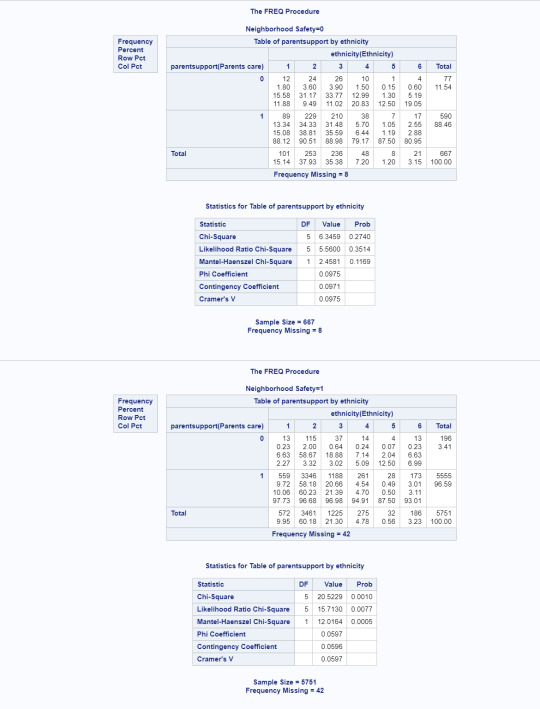
Notable things about initial chi-square results before post-hoc. First, some sample sizes are now incredibly small, which may affect accuracy of results (the group of Native youth in an unsafe neighbourhood is only 4 and Asian youth in an unsafe neighbourhood is only 7). That said, There is obviously something happening here that warrants further testing. All three initial chi-square tests showed a p<.0001. Here, nearly every test has less power than the initial test and the chi-square for parent support for adolescents in unsafe neighbourhoods is no longer significant. 

Selected Post Hoc Test

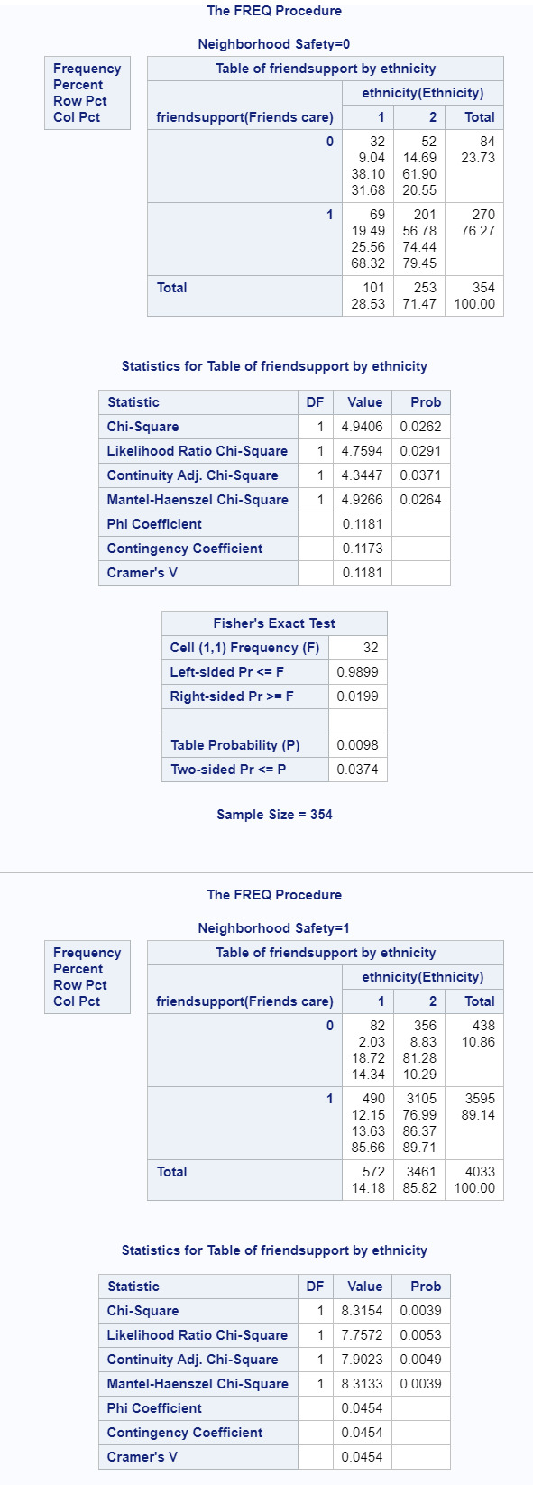
For each protective factor in post hoc testing, alpha has been changed to .003 to compensate for increased Type 1 error. Based on that, it is clear that neighbourhood safety is a moderating factor. Initial results demonstrated a significant association between ethnicity and friend support for mixed and white youth (p<.0001) with 81.99% of mixed youth feeling their friends highly cared about them vs. 88.87% of white youth. Here, when controlling for neighborhood safety, there is no longer an association between ethnicity and friend support for mixed and white youth. I’ve summarized other relevant results below:

Adult Support

Initial results showed that there were significant results for mixed and white youth as previously stated as well as white and Latinx youth (87.42% vs 79.45% p<.0001), white and Asian youth (87.42% vs 77.4%, p<.0001), Black and Latinx youth (86.31% vs 79.45%, p=.0017), and Black and Asian youth (86.31% vs. 77.4%, p=.0007). When controlling for neighbourhood safety, there were no significant results for any youth in unsafe neighbourhoods. In safe neighbourhoods, only two results remained significant. White youth were more likely to feel supported by adults (88.38%) than Asian youth (79.03%), p=.0001. These are both slightly higher percentages than without the neighborhood safety moderating variable. Black youth were also more likely (88.41%) than Asian youth (79.03%) to feel supported by adults, p=.0004. 

Parent Support

Initial chi-square tests without controlling for neighborhood safety showed two significant results: white youth felt more supported than Latinx youth (96% vs 92%, p=.0006) and white youth felt more supported than Asian youth (96% vs 91%, p=.001). Again, once controlling for neighborhood safety, there were no significant results for youth in unsafe neighborhoods. However, in safe neighborhoods, neither of the initial significant results were significant anymore. Three different results became significant:

97.73% of mixed youth felt high support from parents compared to 87.5% of Native youth, p=.0007. This is compared to initial results without neighborhood safety where 95.02% of mixed youth felt supported compared to 87.5% of Native youth (p=.04). 

97.73% of mixed youth felt high support from parents compared to 93.01% of Asian youth, p=.002. This is compared to initial results without neighborhood safety where 95.02% of mixed youth felt supported compared to 91.35% of Asian youth (p=.05).

96.98% of Black youth felt high support from parents compared to 87.5% of Native youth, p=.0029. This is compared to initial results without neighborhood safety where 95.5% of Black youth felt supported compared to 87.5% of Native youth (p=.02).

To summarize, when controlling for neighborhood safety, there is no significant association between ethnicity and parent support in unsafe neighborhoods. In safe neighborhoods, there is a significant association between mixed and Native youth, mixed and Asian youth, and Black and Asian youth and in all three cases, more youth felt supported than when not controlling for neighborhood safety.

Friend Support

Initial chi-square results showed the most significant results between ethnicity and friend result. There were initially five significant results summarized below.

88.87% of white youth felt supported by friends compared to 81.99% of mixed youth with p<.0001

88.87% of white youth felt supported by friends compared to 76.43% of Black youth with p<.0001.

88.87% of white youth felt supported by friends compared to 77.61% of Latinx youth with p<.0001.

88.87% of white youth felt supported by friends compared to 67.5% of Native youth with p<.0001.

88.87% of white youth felt supported by friends compared to 78.85% of Asian youth with p<.0001.

When controlling for neighborhood safety, there was only one significant result in unsafe neighborhoods. 79.45% of white youth in unsafe neighborhoods felt supported by friends compared to only 66.95% of Black youth (p=.0018). 

In safe neighborhoods, all initial significant results remained significant and two additional results became significant:

89.71% of white youth felt supported in safe neighborhoods compared to 85.66% of mixed youth with p=.003.

85.66% of mixed youth felt supported by friends in safe neighborhoods compared to only 78.53% of Black youth with p=.0003.

Overall, because neighborhood safety affected the strength of many of the significant results in each protective factor, it is safe to say that it is a moderating variable for protective factors and ethnicity.

[naduahcoursera]

Pearson Correlation

proc corr; var h1to2 h1to14;

My usual research question does not apply here, so I chose two different quantitative variables from the ADDHealth data set: age of first full cigarette and age of first drink without parents.

Scatterplot

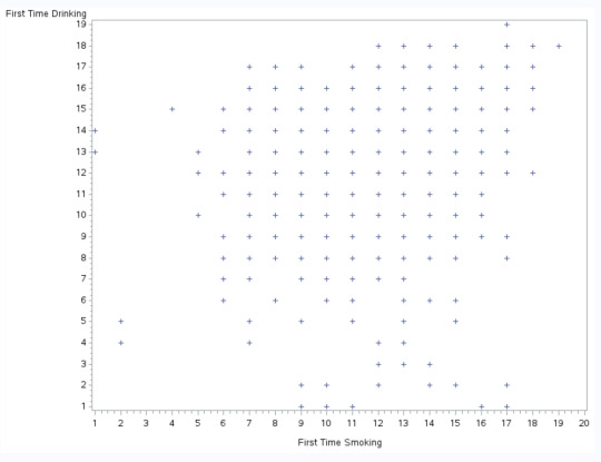
The scatterplot seems to show a somewhat weak positive relationship. I would assume it is somewhat weak because of how widespread all the data points are and they are not congregating around any particular data point. That said, since these are discrete values, a scatterplot would create distinct points rather than clusters anyway.

Correlation Output

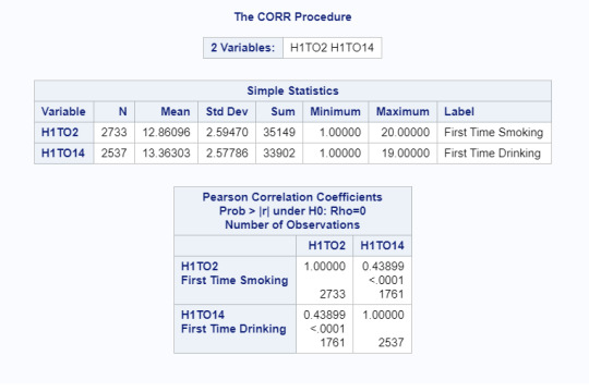
The correlation output confirms a positive association that is stronger than what I initially expected (r=.438), though it’s still not especially strong. It is however statistically significant with p<.0001.

The r^2 is .192, meaning if we know the first time an adolescent had a cigarette, we can predict only 19% of the variability we will see in their first time drinking without parents, which leaves 81% unaccounted for.

[naduahcoursera]

Chi-Square Test

Code for 1 of the 15 post hoc tests

Data comparsion1; set new; if ethnicity=1 or ethnicity=2; proc sort; by AID; proc freq; tables adultsupport*ethnicity/chisq; proc freq; tables parentsupport*ethnicity/chisq; proc freq; tables friendsupport*ethnicity/chisq; run; Data comparsion2; set new;

Initial Chi Square Test

My research question was examining how protective factors questioned in the ADDHealth Study (primarily supportive relationships) were associated with ethnicity. In previous work, I’ve collapsed the protective factor variables into two categories: high care and low care. When running the Chi-Square test, all 3 primary protective factors I’m interested in (adult support, parent support, and friend support) showed significance all at p<.0001 as seen in tables below. 

Because ethnicity has 6 possible values, it was necessary to run post hoc testing for each protective factor. For each protective factor variable, that meant 15 different comparisons, so the significance value was changed to .003 to compensate for increased Type 1 error. Since including every result would be 45 chi-square results, I’ve included one table and have summarized the results for that table.

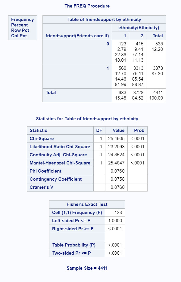
Here, it is clear that we can reject the null hypothesis and there is a significant association (p<.0001) between ethnicity and how much adolescents feel their friends care about them. In this example, only 81.99% of the mixed race youth felt their friends highly cared about them in comparison to 88.87% of white youth. 

Other significant results are as follows:

Adult Support

87% of white youth felt high support from adults compared to 83% of mixed youth with p=.0018.

87% of white youth felt high support from adults compared to 79.45% of Latinx youth with p<.0001.

87% of white youth felt high support from adults compared to 77.4% of Asian youth with p<.0001.

86% of Black youth felt high support from adults compared to 79.45% of Latinx youth with p=.0017.

86% of Black youth felt high support from adults compared to 77.4% of Asian youth with p=.0007.

Parent Support

96% of white youth felt high support from parents compared to 92% of Latinx youth with p=.0006.

96% of white youth felt high support from parents compared to 91% of Asian youth with p=.001

Friend Support

88.87% of white youth felt supported by friends compared to 81.99% of mixed youth with p<.0001

88.87% of white youth felt supported by friends compared to 76.43% of Black youth with p<.0001.

88.87% of white youth felt supported by friends compared to 77.61% of Latinx youth with p<.0001.

88.87% of white youth felt supported by friends compared to 67.5% of Native youth with p<.0001.

88.87% of white youth felt supported by friends compared to 78.85% of Asian youth with p<.0001.

[naduahcoursera]

ANOVA

proc anova; class ethnicity; model h1to2=ethnicity; means ethnicity/DUNCAN;

Model Interpretation for ANOVA:

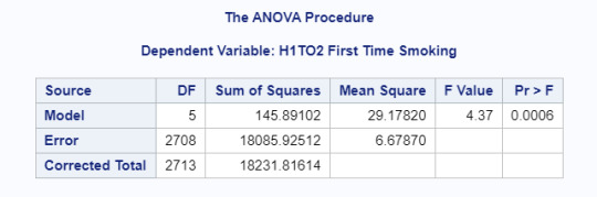
My original research question would not use an ANOVA test because it is a categorical to categorical question. For the purposes of this test, I decided to look at how ethnicity (categorical explanatory variable) is associated with age first started smoking (quantitative response variable). To make the data more manageable, I coded out legitimate skips because youth had never smoked as well as unknown and refused data. I also removed data for those who had never smoked a whole cigarette. The ANOVA revealed that there was a significant association and the null hypothesis could be rejected F(5, 2708)=4.37, p=.0006. As seen in the following table. I did not include individual means because ethnicity is a categorical variable with more than 2 categories and requires further testing to be significant.

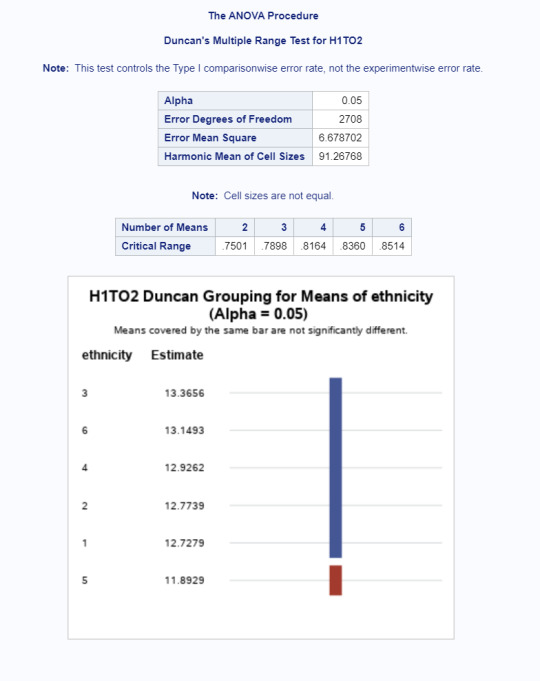
Model Interpretation for post hoc ANOVA results:

Running the Duncan post hoc test showed that Native youth were significantly more likely (p=.0006) to smoke earlier M=11.89 than any other ethnicity. No other comparison was statistically significant as seen in the Duncan output below.

[naduahcoursera]

Graphing Data

Univariate Graph of Ethnicity

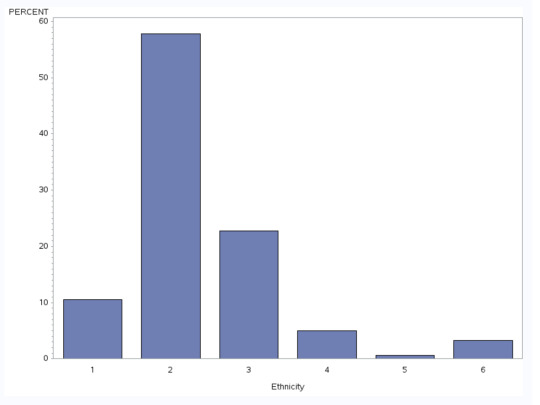
This graph is unimodal with its highest peak at 2, “White”. It is somewhat skewed to the right, but that doesn’t mean very much with a categorical variable.

Univariate Graph of Teachers Caring

This graph has uniform modality. Since it has been collapsed already into two categories, each has nearly 50% of the responses and there is no modality.

Bivariate Graph of Teachers Caring and Ethnicity

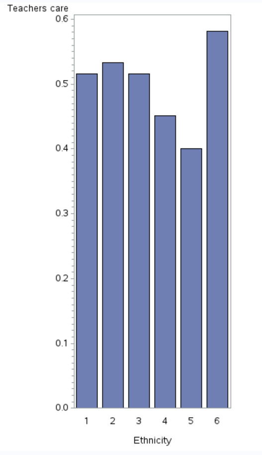
This graph is a C-->C bar chart of ethnicity and teachers caring as a protective factor. There is a slight modality with more Asian and Pacific Islander youth (6) reporting that their teachers cared about them than the other ethnicities. There is a distinct drop for Native youth (5). Further statistical analysis is necessary to determine if this is significant.

Additionally, I did run bivariate graphs for each protective factor variable as seen in the program, but did not place them here because most are almost completely uniform with no distinct modality. Further investigation is necessary before proceeding.

[naduahcoursera]

Data Management Decisions

My research topic is examining how race and protective factors are associated. To make the data more manageable, I created a new ethnicity variable that sorted the ADDHealth individual variables into one aggregate variable. As can be seen in this new variable, 10.58% of youth were mixed race, 57.77% were white, 22.75% were Black or African American, 5.05% were Latinx or Hispanic, only .62% were Native American and 3.22% were Asian or Pacific Islander. This is interesting given my previous focus on either White or Native participants based on personal interest. The previous percentage of Native participants was 3.64%, meaning that it is likely many Native participants marked multiple races, collapsing them into the multi-ethnic category and I will need to evaluate how to manage this discrepancy moving forward. 

For protective factors, I’m aware I have more than 3 variables, but I am working on further condensing all 8 measured protective factors. For now, I collapsed each protective factor into two categories rather than the original 5. I divided each along approximately the same lines to create a “high” and “low” category for each protective factor. For adult support, 85.89% of youth had high support, 52.48% of youth had high teacher support, 95.4% of youth had high parent support, 84.27% of youth had high friend support, 55.46% of youth felt their families had high understanding of them, 63.56% had a low desire to leave home, 62.25% had high ratings of fun with their families and 70.63% of youth had high attention from their families. While I could have divided some of these categories in ways that provided a more even distribution, it felt more important to group similar responses across all variables, rather than choosing each to provide an even distribution. 

[naduahcoursera]

First Program Output

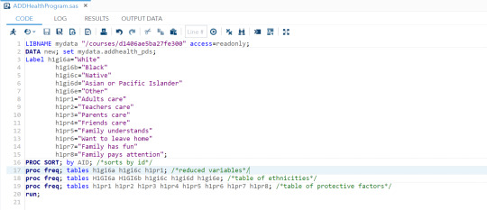
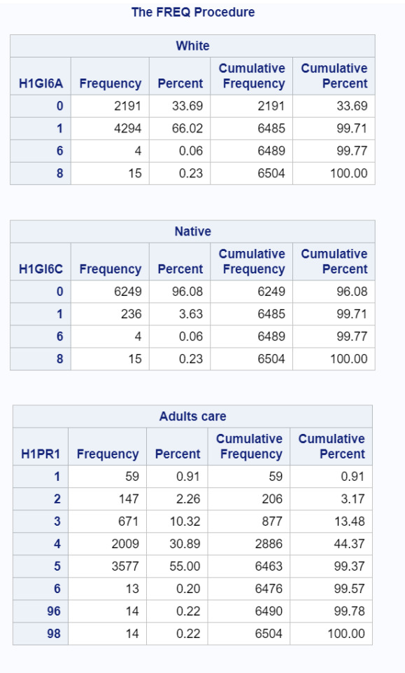
I am interested in looking how protective factors and race are associated in adolescents. For the purposes of this brief assignment, I reduced the total race category variables into the two comparisons I’m primarily interested in, white vs. POC youth and specifically Native youth since I work with homeless Native youth. In my program I left the full list of each variable because I am hoping to aggregate or combine the racial categories into a variable that makes more sense, but am not quite there yet. 

In the frequency tables, 66.02% of the sample were white and 33.69% were not. A tiny percentage (.29% total) either refused or didn’t know. There was a surprisingly large percentage of Native adolescents represented with 3.63%. Overall, with regard to how much the youth felt adults cared about them, the majority  (55%) felt that adults cared about them very much. 30.89% felt that adults cared quite a bit, only 10.32% said adults somewhat cared about them, and 2.26% and .91% felt adults cared about them very little or not at all respectively. A nearly negligible amount didn’t answer the question either because it did not apply (.2%), they refused (.22%), or they didn’t know (.22%).

[naduahcoursera]

Research Question

I chose the ADDHealth dataset because it included information on relationships and social factors, which are both issues I have worked on before. I currently work with Native homeless youth, so this data set also felt the most applicable to my current position and the work I am already doing.

Because I work with Native youth, I am especially interested in how health, social protection, and other variables fall along racial lines. I knew I would begin looking at basic demographic information like race and possibly socioeconomic status, but it took some time to decide what to specifically focus on for the association. I have investigated domestic and sexual violence in the past, so I initially investigated the relationship variables. However, I couldn’t see anything specific that was of interest and eventually decided that rather than looking at violence, I wanted to examine the flipside and decided to see how protective factors were associated with race. 

When looking at the literature, some research looked at this similar comparison of protective factors across entire ethnic groups (Katz et al., 2020), but this research suggested that looking at these issues on a broad scale may not be the most effective and instead, these issues may need to be examined on a family by family or child by child basis. Further research specifically on youth in group homes found that there was a noticeable difference along race-gender lines for both risk and protective factors in the youth studied (Strack et al., 2007). A study by Birndorf et al. (2004) further supported this idea of racial and gender differences, specifically looking at how protective factors affected self-esteem in adolescents. Their study suggested that boys reported higher self-esteem than girls and there were differences across racial/ethnic groups. A study by Davidson and Wingate (2011) added complexity in examining protective factors and race. Looking specifically at protective factors and suicidality, they found that African Americans had more protective factors than their Caucasian counterparts. This adds complexity in that it stands in opposition to much research that suggests that non-White people have fewer protective factors than white people. This study also highlights the importance in defining protective factors for both this study and future research as the factors measured in this study were different than those in the ADDHealth study. Finally, Neblett Jr, Rivas-Drake, and Umana-Taylor (2012) helps to highlight the importance for this research. This study examines protective factors for youth, specifically around racial and ethnic support and reducing discrimination and how improving these factors can improve health and social outcomes for youth.

Ultimately, there are few studies examining a) protective factors across such a wide range of ethnic groups and b) examining these specific protective factors. It deserves to be noted that protective factors is a broad term and the ADDHealth data specifically looked at connections to support by parents, teachers and other adults, which neglects protective factors often described such as religiosity, income, ethnic support, and more. Drawing from the limited research around these topics, my hypothesis is that white adolescents will have higher rates of protective factors than their non-white counterparts. 

Bibliography

Birndorf, S., Ryan, S., Auinger, P., & Aten, M. (2005). High self-esteem among adolescents: Longitudinal trends, sex differences, and protective factors. Journal of Adolescent Health, 37(3), 194–201. https://doi.org/10.1016/j.jadohealth.2004.08.012

Davidson, C. L., & Wingate, L. R. R. (2011). Racial Disparities in Risk and Protective Factors for Suicide. Journal of Black Psychology, 37(4), 499–516. https://doi.org/10.1177/0095798410397543

Katz, B., Turney, I., Lee, J. H., Amini, R., Ajrouch, K. J., & Antonucci, T. C. (2020). Race/Ethnic Differences in Social Resources as Cognitive Risk and Protective Factors. Research in Human Development, 17(1), 57–77. https://doi.org/10.1080/15427609.2020.1743809

Neblett, E. W., Rivas-Drake, D., & Umaña-Taylor, A. J. (2012). The Promise of Racial and Ethnic Protective Factors in Promoting Ethnic Minority Youth Development. Child Development Perspectives, 6(3), 295–303. https://doi.org/10.1111/j.1750-8606.2012.00239.x

Strack, R. W., Anderson, K. K., Graham, C. M., & Tomoyasu, N. (2007). Race–gender Differences in Risk and Protective Factors among Youth in Residential Group Homes. Child and Adolescent Social Work Journal, 24(3), 261–283. https://doi.org/10.1007/s10560-007-0084-y