
Last Seen Blogs

standuphippy
Stand Up, Hippy!

cid-onia
Things That Make Me Happy

ogurgey
Rumblings

kz365247
i wish it were christmas all the time

aboutpreviews
Use aboutp for me to reblog
Text
Capstone Assignment 3: Preliminary Results
Results:
Descriptive Statistics:
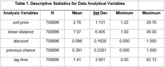
Table 1 shows the descriptive statistics for the quantitative predictors. The average unit price was 2.76 SGD/km (sd=1.131), with a minimum unit price of 1.22 SGD/km and a maximum of 29.76 SGD/km. The other predictors can be interpreted in the same way, according to the data in Table 1.
Table 1. Descriptive Statistics for Data Analytical Variables
Bivariate Analyses:
The response variable is categorical in 2 levels. Therefore, all bivariate analyses will be plotted using bar charts. For the predictors that are also categorical in 2 levels, the following figure, Figure 1, shows the Association between Categorical Predictors and the response variable: the x-axis represents the predictor categories with ‘1’ represents ‘yes’, and ‘0’ represents ‘no’, and y-axis represents the probability of the user to put a request at each category in the x-axis.
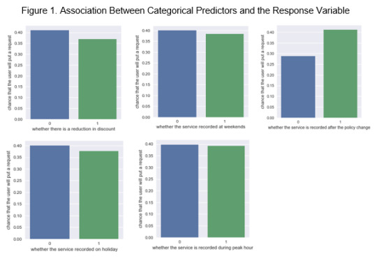
The chi-square tests have been conducted on the above five conditions after plotting the bar charts. It revealed that the customers were more likely to put a request to the Grab taxi service after the policy change than they were before (χ2 = 5244.8, p-value < .0001). But the customers were less likely to put the request if there was a reduction in the discount compared with previous time (χ2 = 1197.8, p-value < .0001), and during public holidays (χ2 = 309.5, p-value = 2.82 x 10-69 < .0001). All the p-values showed that these predictors are significantly associated with the response variable. The last two variables, whether services recorded at weekends and during peak hours, even though showed significant associations with the response variable (weekend: χ2 = 179.8, p-value < .0001; peak hours: χ2 = 30.66, p-value < .0001), the association is not strong enough to make the probability at each category distinguishable. For the predictors that are quantitative, it is necessary to divide the predictors into subgroups and then establish the bar charts. The quantitative predictor, unit price, was taken as an example. From the descriptive statistics data, unit price is categorized into four subgroups: 0~2.245, 2.245~2.415, 2.415~2.732, and 2.732~30 (SGD/km). And the bar chart is plotted and showed in figure 2.
Figure 2. Association Between Unit Price and Response Variable
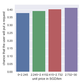
It showed that the customers were more likely to put a request to book Grab service as the unit price increases. This conclusion is not consistent with the common sense, However, since it is only possible to find the association between two variables, not causality. There might be other variables which is confounding to these two variables, further discoveries would be discussed in multivariant model. Then, we run chi-square test again to do the statistical test. Since the categorical predictor has 4 levels, post-hoc test is required.
Table 2. p-values among every comparison for unit price post-hoc test

By adopting the Bonferroni adjustment, the acceptable p-value with 6 comparisons is 0.008. And the results for each pair of the comparisons were smaller than 0.008, which showed the association between unit price and the response variable that was discovered is significant.
The same test was run to find the association between discount and response variable. And the results are shown below:
Figure 3. Association Between Discount and Response Variable

Table 3. p-values among every comparison for discount post-hoc test
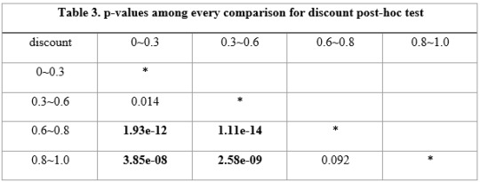
From the post-hoc test results, it revealed that the association between category 0~0.3 and 0.3~0.6 is larger than the adjusted acceptable p-value 0.008. Hence the association between discount and response variable under these two categories is not significantly associated. It also explained why association between these two categories was not consistent with those between other categories. And the association is not significant either falls between 0.6~0.8 and 0.8~1.0. However, the general association between discount and response variable that was proved to be significant was that the customers were more like to put request when the discount is larger (means the value was smaller).
Lasso Regression Analysis:
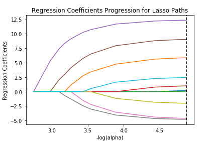
Table 4 and Figure 4 showed that 10 of 10 predictors were retained in the selected model by the lasso regression.
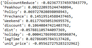
Table 4: Predictors and the Lasso Least Angle Regression Coefficients
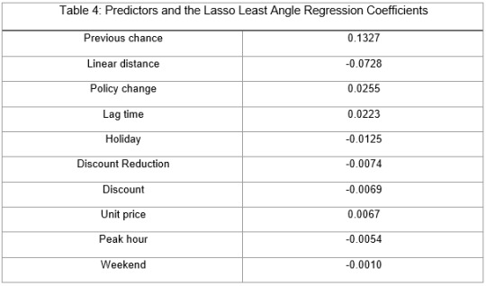
Figure 4 Regression Coefficients Progression for Lasso Paths
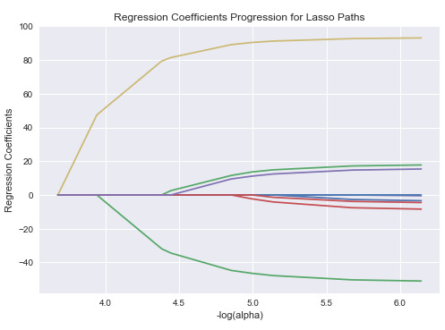
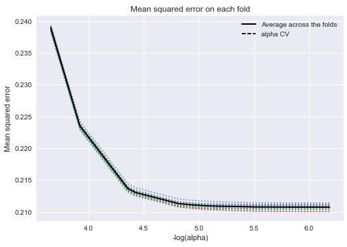
During the estimation process, Previous chance of putting request after open the app was most strongly associated with whether one will put request this time. And they are positively associated. Followed by the linear distance from user’s current location to the destination, which is negatively associated. The strength of the associations can be seen in Table 4, the larger the absolute value of the coefficient means the stronger the association between individual predictor and response variable. The sign indicates the association is positive or negative. These 10 variables accounted for 21.08% of the variance (in Figure 5) in predicting whether the user would put a request to book taxi, which is my response variable.
Figure 5 Mean squared error on each fold
0 notes
Text
Capstone Week 2
Methods Section in my Capstone report draft
Sample:
The targeting population of this study are the customers who have registered Grab mobile account and have at least opened the Grab app on their mobiles. The service record of each customer during each time of the service has been stored in Grab server. And the sample of this study was extracted to include N=708896 customers’ latest records, through a wide range of days, from June 1, 2016 to September 20, 2016. Each record belongs to only one customer and only the latest record of each customer would be extracted in the sample. The sampling date also crosses the date August 27, 2016, on which there was a policy change in Grab company.
Measures:
The user’s final decision on whether to put a request to book the taxi using Grab app is the categorical response variable, which is recorded down each time after the users have opened the Grab app on their mobiles (yes/no).
Predictors included 1) unit price: the cost in Singapore dollars (SGD) the user need to pay per kilometre for the service, 2) linear distance: the linear distance from the user’s current location to the destination in kilometres, 3) discount: the cost that is being deducted during promotion for the current service in SGD, 4) discount reduction: the discount from last service, if there is, is used to be compared with the current discount, to see if there is a reduction in discount (yes/no), 5) previous chance of putting a request after open the app: it is obtained by using the number of requests the user has sent divided by the number of how many times the user has opened the Grab app (, the variable names can be found in the appendix codebook ), 6) policy change: whether the service record is after the date on which the policy was changed (yes/no), 7) lag time: how long it has been since the last time the user opened the Grab app, 8) holiday: whether the service is recorded on public holiday (yes/no), public holidays is defined in terms of Singapore public holiday based on the local culture, 9) weekend: whether the service is recorded at weekends (yes/no) 10) peak hour: whether the services recorded is during peak hours (yes/no), peak hours are defined as: 7 a.m. to 9 a.m.(end points inclusive) and 5 p.m. to 8 p.m.(end points inclusive) at local time.
Analyses:
The distributions for the predictors and the user’s final decision on sending the request, the response variable, were evaluated by examining frequency tables for categorical variables and calculating the mean, standard deviation and minimum and maximum values for quantitative variables.
Bar charts were also examined, and Chi-Square Test and post-hoc test were used to test bivariate associations between individual predictors and the categorical response variable, which is user’s decision on whether to put request to the service.
Lasso regression with the least angle regression selection algorithm was used to identify the subset of variables that best predicted whether the user is going to put a request to the Grab service. The lasso regression model was estimated on a training data set consisting of a random sample of 70% of the service records (N=496227), and a test data set included the other 30% of the service records (N=212669). All predictor variables were standardized to have a mean=0 and standard deviation=1 prior to conducting the lasso regression analysis. Cross validation was performed using k-fold cross validation specifying 10 folds. The change in the cross validation mean squared error rate at each step was used to identify the best subset of predictor variables. Predictive accuracy was assessed by determining the mean squared error rate of the training data prediction algorithm when applied to observations in the test data set.
0 notes
Text
Capstone Week 1
My project Title:
An Algorithm for Predicting Grab User Booking Behavior to Maximize Profit
Introduction to the Research Question:
(research question)
The purpose of this study was to identify the significant factors that are associated with the user’s choice of putting a request to book the taxi via Grab mobile app. The aim was that by focusing on these factors or variables such as unit price, recent discount, distance from destination, and previous behavior patterns, one could be able to predict whether there is a higher or lower chance for the customer to book the taxi service using the Grab app.
(motivation & rationale)
Instead of calling for normal taxi, there must be more that Grab could offer when one choose to use Grab mobile app to book the service. From the Grab company’s perspective, it is important to have a better understanding of factors that are most likely to affect users’ final decision on requesting services. And this enables decision makers in Grab to focus on those significant and tune-able factors to maximize the profit for the company.
(potential implications)
Predictable customer behavior pattern can help Grab build more profitable and customized algorithms. Meanwhile, it would also satisfy customers’ desire by providing reasonable price and fair discounts under different circumstances when the service is requested.
0 notes
Text
Course4 Assignment4 Running a K-Means Cluster Analysis
A k-means cluster analysis was conducted to identify underlying subgroups of Grab app users based on their similarity of responses on 5 variables that represent characteristics that could have an impact on whether they would choose to put a request to book a taxi at current time. Clustering variables included 5 quantitative variables, such as unit price for the service, how much discount the user could have for this booking request, the linear distance between current location and the destination, previous chance of putting a request after opening the app, and how long it has been since last time of using the Grab app. All clustering variables were standardized to have a mean of 0 and a standard deviation of 1.
Data were randomly split into a training set that included 70% of the observations (N=7227) and a test set that included 30% of the observations (N=3097). A series of k-means cluster analyses were conducted on the training data specifying k=1-9 clusters, using Euclidean distance. The variance in the clustering variables that was accounted for by the clusters (r-square) was plotted for each of the nine cluster solutions in an elbow curve to provide guidance for choosing the number of clusters to interpret.
Figure 1. Elbow curve of r-square values for the nine cluster solutions
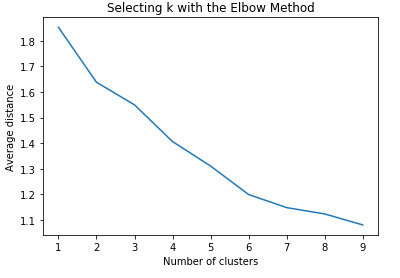
The elbow curve was inconclusive, suggesting that the 2, 3 and 4-cluster solutions might be interpreted. The results below are for an interpretation of the 4-cluster solution.
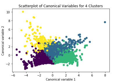
Canonical discriminant analyses was used to reduce the 5 clustering variable down a few variables that accounted for most of the variance in the clustering variables. A scatterplot of the first two canonical variables by cluster (Figure 2 shown below) indicated that the observations in clusters green, blue, and purple were densely packed with relatively low within cluster variance, but did overlap very much with the other clusters. Cluster yellow was generally distinct, but the observations had greater spread suggesting higher within cluster variance. Observations in cluster yellow were spread out more than the other clusters, showing high within cluster variance. The results of this plot suggest that the best cluster solution may have fewer than 4 clusters, so it will be especially important to also evaluate the cluster solutions with fewer than 4 clusters.
Figure 2. Plot of the first two canonical variables for the clustering variables by cluster.
Hence, 3 clusters were adopted and plotted in Figure 3:
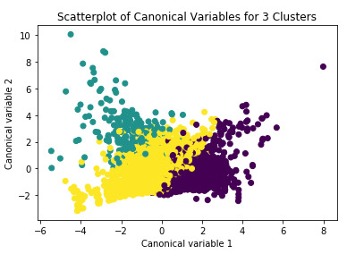
Figure 4:
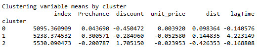
The means on the clustering variables showed that, compared to the other clusters, Grab users in cluster 1 had higher chance of booking a request after open the app previously, and had lowest unit price for the service, and logest distance to their destination, and haven’t used the app for a long time. Where as users in cluster 0 has the lowest discount and highest unit price. Therefore, users would not likely to book the service under these circumstances.
In order to externally validate the clusters, an Analysis of Variance (ANOVA) was conducting to test for significant differences between the clusters on a categorical variable, which is whether the user would put a request to book the taxi at current time. A tukey test was used for post hoc comparisons between the clusters.
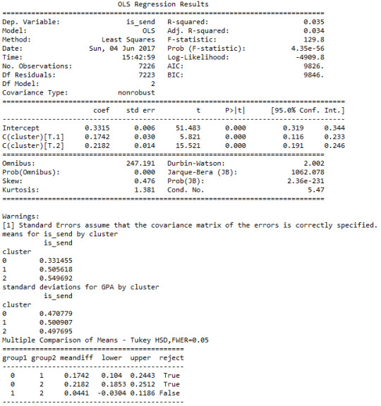
Results indicated significant differences between the clusters on is_send (F(3, 10324)=129.8, p<.005). The tukey post hoc comparisons showed significant differences between clusters on is_send, with the exception that clusters 1 and 2 were not significantly different from each other. Users in cluster 0 had the lower chance of booking a taxi (mean=0.33, sd=0.47), and cluster 2 had higher chance of putting a request (mean=0.55, sd=0.50).
0 notes
Text
Course4 Assignment3 Running a Lasso Regression Analysis
A lasso regression analysis was conducted to identify a subset of variables from a pool of 10 categorical and quantitative predictor variables that best predicted a categorical response variable which is whether the use will put a request after open the Grab app.
Categorical predictors included whether it is a holiday, whether it is a weekend, whether it is during peak hours, and if the situation where it is before or after Grab policy being changed. Quantitative predictor variables include unit price, distance between where they are and the destination they want to go to, how much discount is provided, what is the chance that they put request after open the app, and how long it has been since one opened the app last time. All predictor variables were standardized to have a mean of zero and a standard deviation of one.
Data were randomly split into a training set that included 70% of the observations (N=7227) and a test set that included 30% of the observations (N=3097). The least angle regression algorithm with k=10 fold cross validation was used to estimate the lasso regression model in the training set, and the model was validated using the test set. The change in the cross validation average (mean) squared error at each step was used to identify the best subset of predictor variables.
Figure 1. Change in the validation mean square error at each step

Of the 10 predictor variables, 8 were retained in the selected model.
During the estimation process, Previous chance of putting request after open the app was most strongly associated with whether one will put request this time(purple line, 0.145), followed by how much is the discount(brown line, 0.106). Whether before or after policy change and the lionear distance between current location and the destination comes next with(orange line, 0.069, and grey line, -0.058), meaning that linear distance is strongly negatively associated with whether the user will put a request and policy change were positively associated with whether to put a request to book the taxi. Other predictors associated with higher chance for one to put a request included unit price(-0.056), how long it has been since last time opened the app and if the discount has been reduced from the last time. These 8 variables accounted for 17.9% of the variance in predicting whether the user would put a request to book taxi, which is my response variable
0 notes
Text
Course4 Assignment2 Running a Random Forest
I have changed my data set. The data collected is the recording of user’s choices of whether to put a request of booking grab taxi depending on the current many variables: distance, discount, effect of policy change, whether it is peak hour, whether it is weekend, and so on. It is included in the new codebook:
Random forest analysis was performed to evaluate the importance of a series of explanatory variables in predicting a binary, categorical response variable. The following explanatory variables were included as possible contributors to a random forest evaluating whether the user will put a request to book the taxi (my response variable), unit price, distance between where they are and the destination they want to go to, how much discount is provided, what is the chance that they put request after open the app, whether it is a holiday, whether it is a weekend, whether it is during peak hours, is the situation recorded before or after Grab policy changing.
And here is the result:
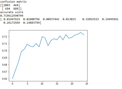
The explanatory variables with the highest relative importance scores were pre chance(0.329), unit price(0.262), discount(0.195) and distance(0.149). The accuracy of the random forest was 72%, with the subsequent growing of multiple trees rather than a single tree, adding more and more to the overall accuracy of the model, and suggesting that interpretation of a single decision tree may not be appropriate.
0 notes
Text
Course4 Assignment1 Running a Classification Tree
I have changed my data set. The data collected is the recording of user’s choices of whether to put a request of booking grab taxi depending on the current many variables: distance, discount, effect of policy change, whether it is peak hour, whether it is weekend, and so on. It is included in the new codebook:
I have run a logistic model that can give me a hint of which explanatory variables have larger effect on the target variable. which is whether the request is sent or not.
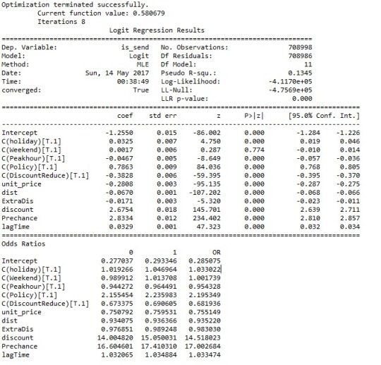
From the result, we can see “discount”, “Prechance”, “Policy” tend to have a positive association with the response variable; whereas “Discountreduce”, “unit price”, “distance”, “Peakhour” shows negative association with the response variable.
Then I run a decision on the three binary explanatory variables “X[0]=‘Peakhour’”, “X[1]=‘Policy’”, “X[2]=‘holiday’”
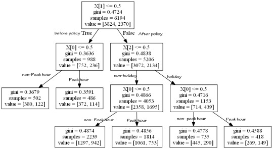
Whether the booking is before or after the policy was the first variable to separate the sample into two subgroups. Then separated by peak hour and holiday. Observations tends to put a request with 75.7% chance before the policy change during the peak hour.
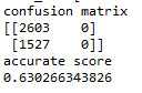
The result is divided into three subgroups by the variables and by printing the confusion matrix, we can see the total model classified 63% of the sample correctly.
The above are all binary variables. If I try to add in one more quantitative explanatory variable, the tree can grow extremely big: (exmaple when I add one more variable “discount”)

Hence I am wondering if the decision tree is meant to find unlinear relationships between quantitative variables and response variable.
1 note
·
View note
Text
Course 3 Assignment 4 Test a Logistic Regression Model
The first topic: The more people care to maintain their social relations (attend important or pleasurable activities) with their colleagues and friends, more likely the failure of cutting down on alcohol would occur. Or the other way around, higher the chance of failing to cut down on the alcohol, more difficult it would be for people to maintain a healthy social or family relation. Therefore, since we cannot determine causality from the regression model, I am just going to check the association between them.
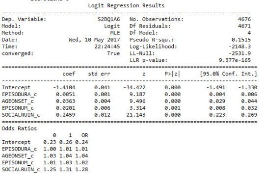
The output the logistic model shows:
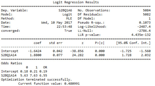
After adjusting for potential confounding factors (list them), the odds of having more than once unsuccessfully tried to cut down on alcohol were more than six times higher for participants who are willing to cut down important meetings to drink than for participants without who are not (OR=6.55, 95% CI = 5.63-7.63, p=.0001).
And after adding the potential confounding variable, from the result:
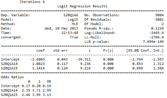
It can be seen that “willingness to give up pleasurable activities to drink” is also significantly associated with whether more than once failed to cut down on alcohol, such that participants who are willing to give up pleasurable activities to drink were significantly more likely to keep failing to cut down on drinking (OR= 3.13, 95% CI=2.46-3.99, p=.0001), and the previous variable is still significantly associated by the odds ratio decreased from 6.55 to 2.95, with its CI in range 2.35-3.71.
To further explore the association, I added more quantitative variables in the logistic model, and here is the result:
It can be concluded that even though the p-values for all the variables are 0.0001. The odds ratios for each of all the explanatory variables approximately are equal to 1, which is indicating that they are not statistically significant. I think this is an inconsistency. Anyone can help explain what does this result really mean?
0 notes
Text
Course 3 Assignment 3 Test a Multiple Regression Model
Today I am focusing on building a multiple regression model:
I want to examine the association between how much a person’s social relationship has been ruined due to alcohol, which is my response variable, and four explanatory variables, which are whether have more than once tried to cut down alcohol (categorical explanatory variable), number of episodes experienced, duration of the longest episodes experienced, and age at onset of alcohol dependence (which are all quantitative explanatory variables).
The response variable is a secondary variable, created by using the occurrences of 4 situations. It is scaled from 0 to 10, and a higher value represents that more severe the person’s social relations have been ruined by alcohol.
After first, I build a linear regression model on all the explanatory variables, and have this results:
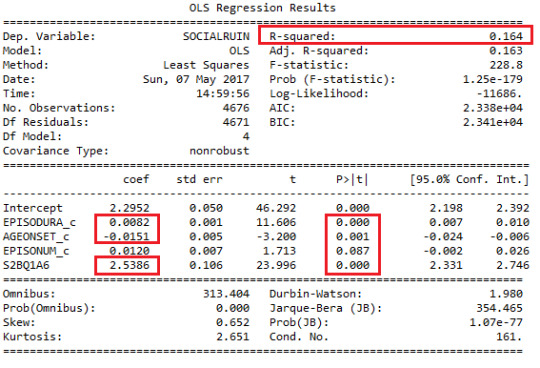
From the result, I can see three of the four explanatory variables shows significant association with the response variable. Among them, the duration of the longest episode and whether more than once failed to cut down on drinking are positively associated with the severeness of how bad the social relations have been ruined (with all p-value = 0.0001). While the age at onset of alcohol dependence is negatively associated with the response variable due to the negative t value and small p-value equals to 0.001 which is smaller than 0.005. However, we can see the number of episodes is not significantly associated with the severeness of how bad the social relations have been ruined, since p-value = 0.087. And its 95% confidence interval also includes 0 which is consistent with the finding. All the three explanatory variables are proven to be significantly associated with response variable by controlling other variables at their mean.
Now, I will plot regression diagnostic plots to examine how well my model can predict the sample. And we can see from previous result, the R-square value is 0.164, which means the explanatory variables can explain only 16.4% of variability in the response variable.
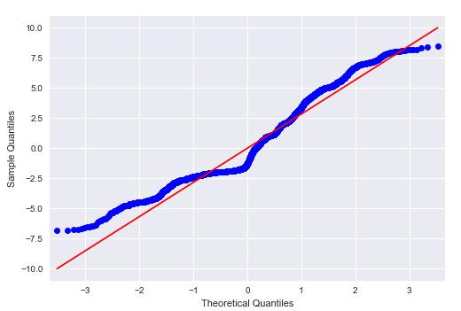
Here is the q-q plot result:
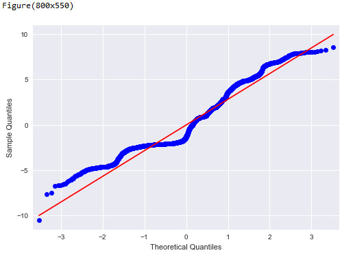
We can see the parameter estimation is not predicting responses well, since the residuals seem not to be normally distributed.
Standardized Residuals for all observation:
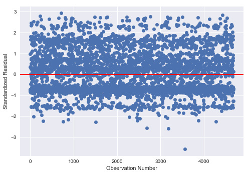
We can observe that there is absolutely more than 5% of the observations has standardized residuals with an absolute value of greater or equal than 2 sigma. And also more than 1% that with value of larger than 2.5 sigma. Hence there’s evidence that the level of error within my model is unacceptable.
I plot partial regression plot on the three significant explanatory variables,
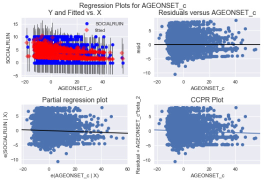
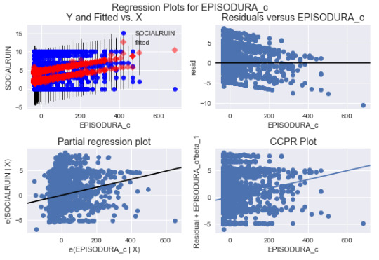
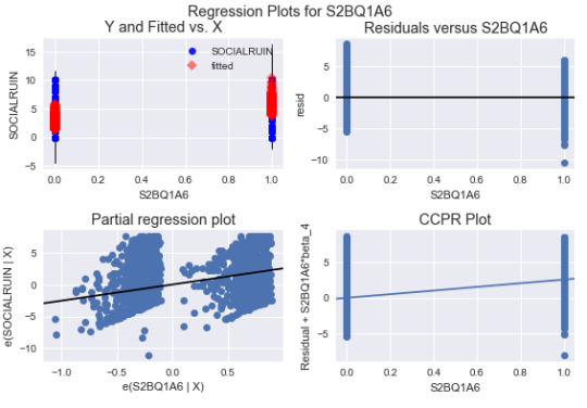
and I can see they are randomly appeared and not showing any curved relationship. It makes me wonder if it is necessary to add quadratic terms of any of the explanatory variables.
leverage plot:
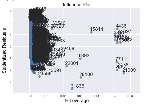
It seems the outliers (those fell out of the -2 ~ 2 std error region) also have a high leverage values. Therefore, these outlying observations do have an undue influence on the estimation of the regression model and therefore should use the flowchart to deal with them.
More experiments:
Add in quadratic term of duration of the longest episode, examine the output:
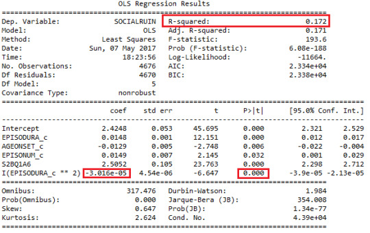
The coefficients have changed for different explanatory variables. And we can see quadratic term of duration of longest episode experienced has a p-value=0.0001, which mean it is significant associated to the response variable. And it is negatively associated as the t value is negative. However, the coefficient is small, around -0.00003, which means the association is quite weak. The improvement of the model is that, R-square increased to 0.172 from 0.164, indicating that the explanatory variables now can explain 17.2% of the variability of the response variable.
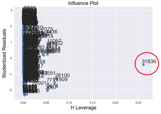
After examine the leverage plot, one large leverage value is obvious to see but not outlier. There are still many outliers but cannot see the leverage value clearly. It seems that the model now improves.
And here is the q-q plot, not much change
Then I keep adding in other quadratic terms for other explanatory variables,
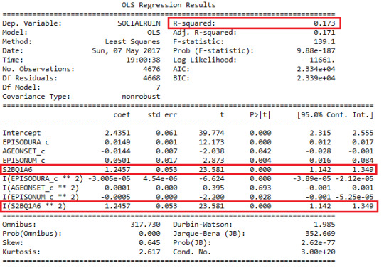
and finding out that quadratic terms for the age at onset of alcohol dependence and the number of episodes experienced are not significantly associated with response variable due to their large p-value.
And obviously, adding higher order term of categorical explanator variable is redundant. Even though with a significant p-value, it is still meaningless to add in collinearity into the model
0 notes
Text
Course3 Assignment2 Test a Basic Linear Regression Model
In this week’s session, I want to build a basic linear regression model using only one explanatory variable and one response variable. And I want to choose explanatory variable under two cases:
Case 1: both explanatory and response variable are quantitative:
Explanatory variable: the age at onset of alcohol dependence (in yrs)
Response variable: Duration of the longest episode experienced (in months)
Using the following code:
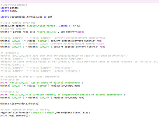
Here is the output:
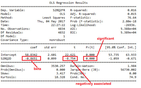
I conclude that the results of the linear regression model indicate that Age at onset of alcohol dependence (beta= - 0.87, p=0.0001) was significantly and negatively associated with the duration of the longest episode experienced. The relation can be expressed as: Y= 58.83 – 0.087X, where X is explanatory variable and Y is response variable.
Case 2: explanatory variable is categorical, response is quantitative
Explanatory variable: more than once unsuccessfully tried to cut down on alcohol (Yes=1 No=0)
Response variable: Duration of the longest episode experienced (in months)
Altering the code like this
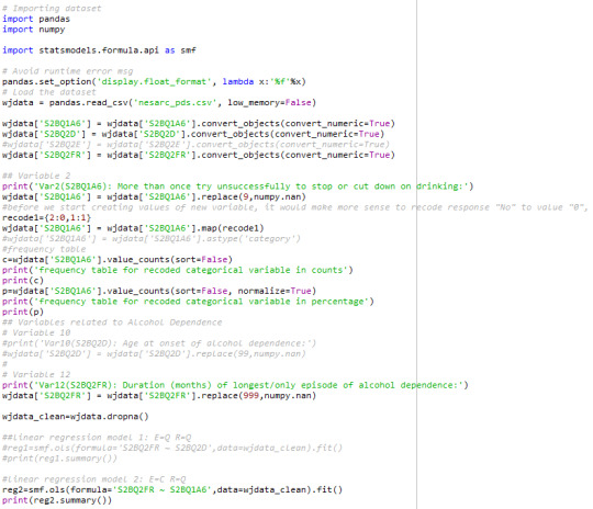
will give the result like following with the frequency table of the recoded categorical variable:
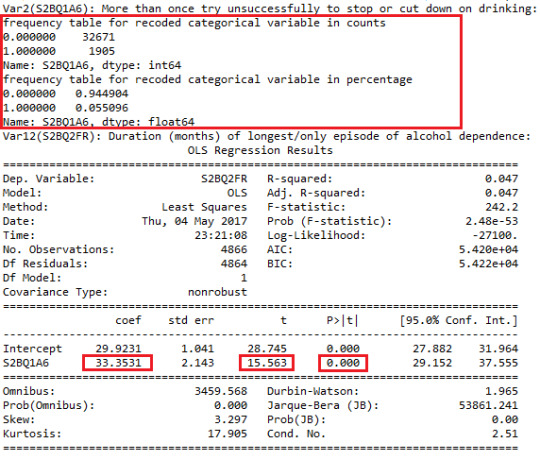
Since now the X is categorical variable, as the video has explained: the result can show us the mean value of the duration of longest episode experienced under two categories: Whether or not more than once unsuccessfully tried to cut down on alcohol? That is using the formula we obtain: Y = 33.35 X +29.92. For group that answers “No”: mean (X=0) = 29.92 and for group that answers “Yes”: mean (X=1) = 63.27. It can be proved consistence with the plot I have plotted out at Course 1 Assignment 4.
0 notes
Text
Course 3 Assignment 1 Writing About Your Data
Step 1: Sample
The sample that I am studying is from the first wave of National Epidemiologic Survey on Alcohol and Related Conditions (NESARC). This survey is focused on the alcohol and drug use and associated psychiatric and medical comorbidities. The targeting population is the civilian, non-institutionalized adult in the United States, including those who live in households, military personnel living off base, and those who are residing in the following group quarters: boarding or rooming houses, non-transient hotels and motels, shelters, facilities for housing workers, college quarters, and group homes. There are totally 43,093 participants who conducted the survey. (N=43,093) The sample I am using for my analysis include all participants who are alcohol dependent, aka. not a lifetime abstainer who has not met symptom and/or duration criteria for lifetime alcohol dependence. (N=5,098)
Step 2: Procedure
The Data was generated by the most common method, which is through sample survey, participants were interviewed by trained U.S. Census Bureau Field Representatives during 2001–2002 through computer-assisted personal interviews (CAPI). The origin purpose of the data collection was to examine the alcohol and related conditions. When the data was collected, one adult was chosen to be interviewed in each household, and interviews were conducted in respondents’ homes following informed consent procedures.
Step 3: Measures
Alcohol dependence (i.e. those experienced in the past 12 months and prior to the past 12 months) was assessed using the NIAAA, Alcohol Use Disorder and Associated Disabilities Interview Schedule – DSM-IV (AUDADIS-IV) (Grant et al., 2003; Grant, Harford, Dawson, & Chou, 1995). The alcohol dependent symptoms of the AUDADIS-IV contain detailed questions on the onset age, number of episodes, and duration in months of longest episode experienced as well as symptom criteria for DSM-IV alcohol dependence.
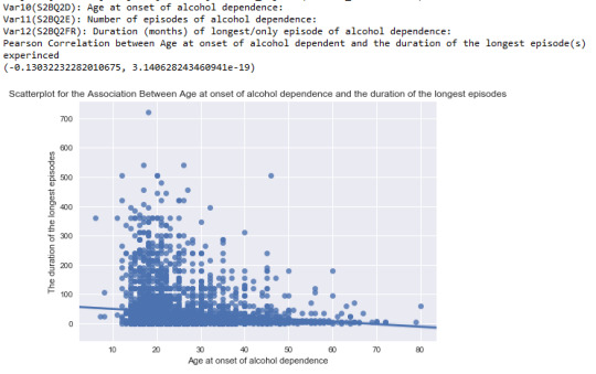
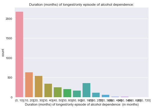
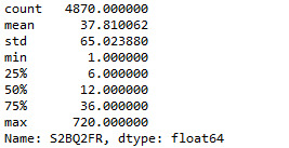
The alcohol dependence was evaluated through onset age of the participant (“Age at onset of alcohol dependence?”) coded to as quantitative variable “S2BQ2D” that ranged from 6 years old up to 98 years old, and the duration of the longest episode(s) experienced (“Duration (Months) of longest/only episode of alcohol dependence?”), also as a quantitative variable “S2BQ2FR” that ranged from 1 month up to 720 months. Some moderators that I think would affect these two variables have been considered, for example: whether the participant who are alcohol dependent have desire to cut down on alcohol. This data is collected in the interview by asking “More than once try unsuccessfully to stop or cut down on drinking?”. This variable is coded as categorical variable which only contains two levels (Yes or No).
0 notes
Text
Course 2 Assignment 4 Testing a Potential Moderator
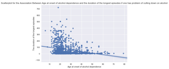
Today, I am focusing on run a Pearson Correlation test that includes a moderator. The case I am using is the same as Assignment 3. I want to discover the relationship between age at onset of alcohol dependence and the duration (in months) of the longest episodes experienced.
From Assignment 3, the results gave me that Pearson Correlation between these 2 variables is -0.13 with a very small p-value indicating that the founding is significant, however, the relation is relatively weak since r is very close to 0. As the following graph shows:
And today, I am thinking a moderator that may effect the direction or strength of the relationship between age at onset of alcohol dependence and the longest episode duration, which is whether the people have problem of cutting down on alcohol.
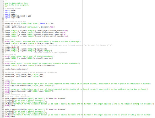
Hence, I use the third variable as a categorical variable and do the following code:
And the results for two subgroups are shown below:
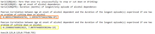
1. Pearson Correlation between age at onset of alcohol dependence if one has no problem of cutting down on alcohol;
2. Pearson Correlation between age at onset of alcohol dependence if one has problem of cutting down on alcohol;
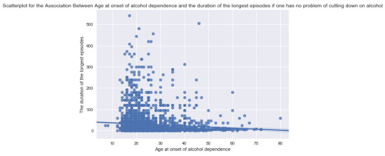
It shows that for the subgroup that having no problem of cutting down on alcohol gives r = -0.086, whereas the subgroup having trouble in cutting down on alcohol gives higher coefficient r = -0.259. Both are with a very significant p-value which is quite small. Showing that for the group of people who have more than once failed to cut down on alcohol tends to have stronger relationship between age at onset of alcohol dependence and the duration of longest episode. But the moderator doesn’t change the direction of the correlation, which is younger people are onset, longer duration of episodes they will experience.
Following are the scatter plots for both of the cases:
0 notes
Text
Course 2 Assignment 3: Generating a Correlation Coefficient
This week I focus on numerically analyzing the relationship between two quantitative variables:
In my case it’s between:
1. “Age at onset of alcohol dependence” and “The number of episodes experienced” or
2. “Age at onset of alcohol dependence ” and “The duration of the longest episodes experienced”
Here is the code I have programmed:
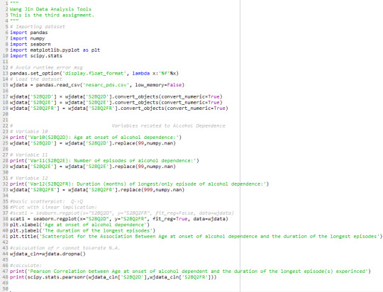
After viewing the first output
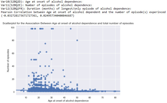
The pearson correlation between “Age at onset of alcohol dependence” and “The number of episodes experienced” is negative: -0.033 with it’s p-value equals to 0.025 proving that r=-0.033 is significant. However, since -0.033 is closer to 0 rather than 1, this negative relations between “Age at onset of alcohol dependence” and “The number of episodes experienced” is weak;
the output of second relationship between “Age at onset of alcohol dependence ” and “The duration of the longest episodes experienced”

The pearson correlation between “Age at onset of alcohol dependence” and “The duration of the longest episodes experienced” is also negative: the older people are onset of alcohol dependence, shorter the duration the episodes would be experienced. r = -0.13 with it’s p-value equals to 3.14e-19 proving that r=-0.13 is very significant. However, since -0.13 is closer to 0 rather than -1, this negative relations between “Age at onset of alcohol dependence” and “The number of episodes experienced” is relatively weak, but stronger than the relation between “Age at onset of alcohol dependence” and “The number of episodes experienced”
After calculating its coefficient of determination
r^2=0.169 which means that if we know the age at onset of alcohol dependence, we can predict 16.9% of the variability we will see in the duration of the longest episodes experienced.
0 notes
Text
Course 2 Assignment 2 Chi-Square test of independence
Model Interpretation for post hoc Chi-Square Test results:
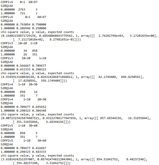
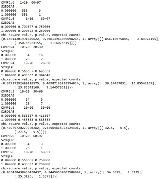
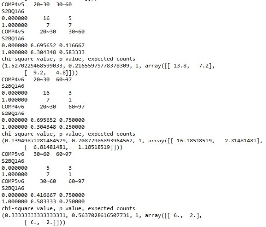
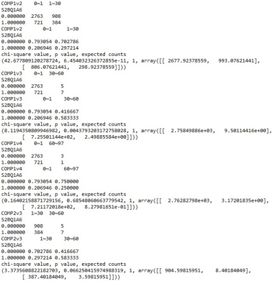
I want to use Chi Square test of independence method to discover if there exists an association between the number of episodes (collapsed into 6 ordered categories) and whether more than once unsuccessfully tried to cut down on alcohol (binary categorical response variable). A post hoc test is required since the explanatory variable has more than 2 levels. For the existing 6 levels, a Chi-Square test between each of the two categories was performed. And there are totally 15 comparisons. The result is shown here:
After making a summary of all the family-wise p-values in a table:
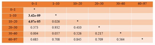
Adjusted Bonferroni p-value: <0.003 (since there are totally 15 comparisons) means that there is statistically significant evidence that these two variables has a relationship, so that we cannot reject the null hypothesis.
The results showed that:
Post hoc comparisons of rates of unsuccessfully tried to cut down on alcohol revealed that those who experienced smaller number of alcohol dependence (group:1 episode) tends to have less rate of unsuccessfully tried to cut down on alcohol than those who experienced more number of episodes of alcohol dependence (group2: 1~10 episodes and group3: 10~20 episodes). The Chi-Square and p-value are respectively: χ2 = 34.93, p = 3.42 x 10⁻⁹; and χ2 = 16.84, p = 4.07 x 10⁻⁵. The associations between other groups are not found statistically significant, since all the other p-values > 0.003.
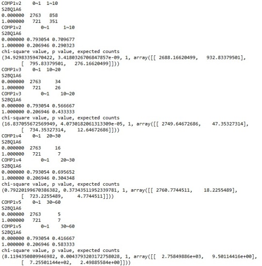
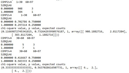
In addition, I also want to discover the effects of how I group the explanatory variable, the number of episodes of alcohol dependence. Hence I decrease the number of categories, from 6 levels to 4 levels. The results are shown below:
After making the p-value summary table:
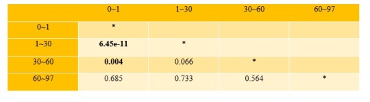
Adjusted Bonferroni p-value: <0.008 (since there are totally 6 comparisons) means that there is statistically significant evidence that these two variables have an association. Thus, we can reject the null hypothesis and say two variables are statistically related.
I found out that p-values between same grouping categories remain the same. But I don’t know how to explain this:
Even though p-value between 0~1 and 30~60 is still 0.004, it is now determined to be statistically significant because the number of comparisons reduced from 15 to 6. It is not the case where the categorical has 6 levels. Need help please.
0 notes
Text
Course 2 Assignment 1
Model Interpretation for ANOVA:
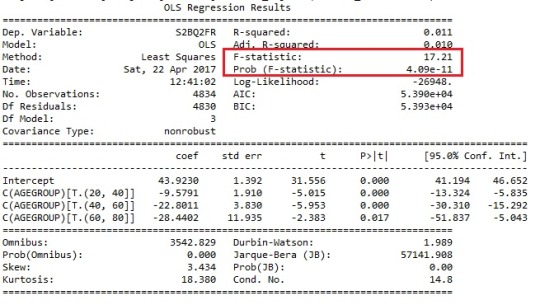
When examining the association between the duration of the longest episode of alcohol dependence (quantitative response) and the age at onset of alcohol dependence (categorical explanatory), an Analysis of Variance (ANOVA) revealed that the younger the participants are onset of alcohol dependence, longer the duration of their longest episode of alcohol dependence would be. According to the age categories: the duration of the longest episode in months is (Mean=43.9, s.d. ±70.96) for age group 5~20 years old; the following groups are listed below:
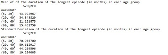
The ANOVA F-test gives the value of F to be F-statistic=17.21, p<0001(4.09e-11).
Model Interpretation for post hoc ANOVA results:
Post hoc test is required, since categorical variable has 4 groups. The p-value cannot provide sufficient guidance anymore. ANOVA revealed that the age at onset of alcohol dependence (collapsed into 4 ordered categories, which is the categorical explanatory variable) and the duration in months of the longest episode (quantitative response variable) were significantly associated.
Post hoc comparisons of mean duration in months of the longest episode experienced revealed that those individuals who are onset alcohol dependence between age 20 to 40 years old reported significantly to experience 18.9 months less than those who are onset between 60 to 80. Category 5~20 and 40~60 were statistically significant associated with group 60~80 as well.
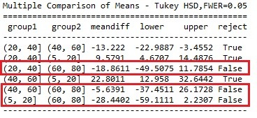
P.S. However, associations among other 3 groups are not statistically significant. In the words, the null hypothesis between 5~20 and 20~40, 5~20 and 40~60, and 20~40 and 40~60 could not be rejected, thus no association found. So in this case, can I still say the duration of the longest episode is associated with the age at onset of alcohol dependence?
0 notes
Text
Assignment 4_Visualizing Data
This week, the focus is on visualizing the selected variables:
Section 1: Creating Univariate Graph for selected variables:
Categorical data:
Variable 1: More than once want to stop alcohol (Yes=1, No=0)
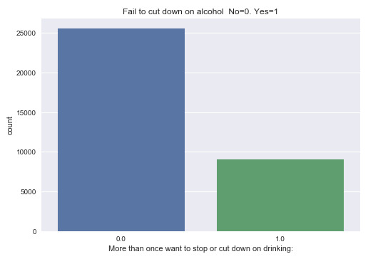
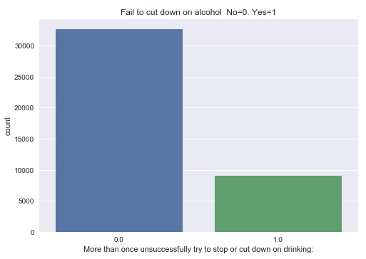
Variable 2: More than once unsuccessfully tried to cut down on alcohol (Yes=1, No=0)
Quantitative data:
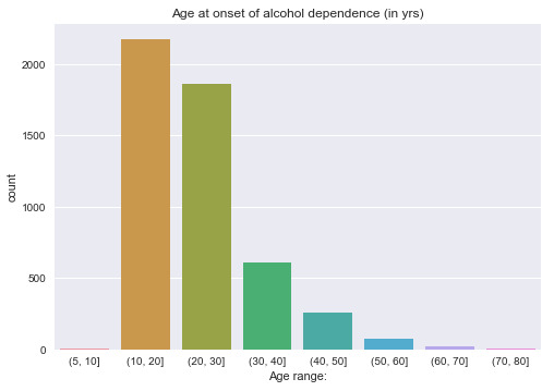
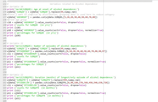
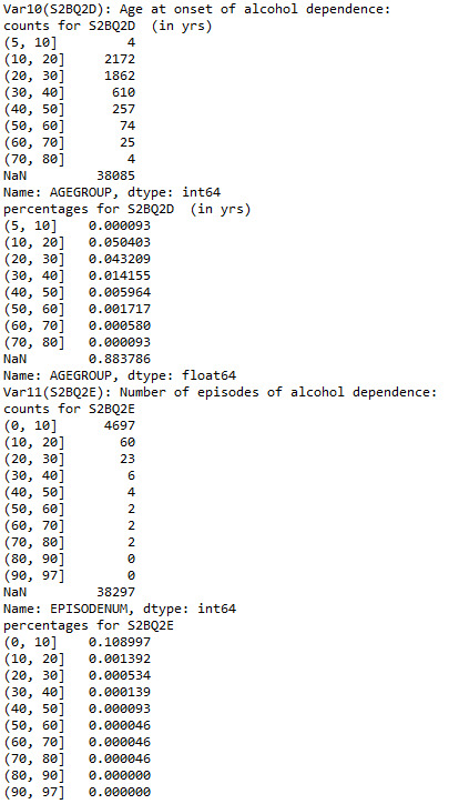
Variable 10: Age at onset of alcohol dependence (in yrs)
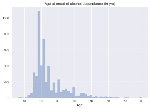
However, we can see if it is plotted as quantitative data, the age range is relatively small, and the observation number under some age range is quite low. For better visualization, I try to plot it after grouping the data, as a categorical data:
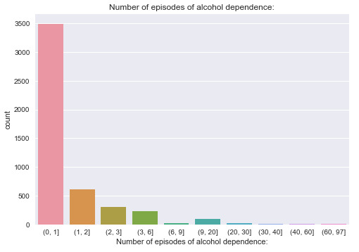
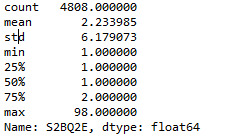
Variable 11: Number of episodes of alcohol dependence
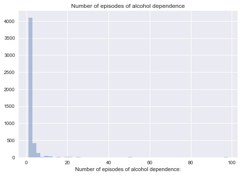
Similarly, I also plot it as categorical data to see through which way it can be visualized better.
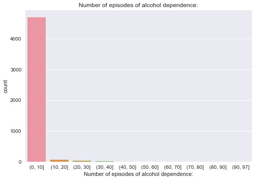
From it, it can be seen most of the data is concentrated in the range of (0,10]. Therefore, I further expand the first category and get the new grouping.
To measure the center and spread, I apply describe function to the quantitative variables:
Variable 9: Created variable to reveal the severity of how bad the social relations have been ruined:
Here is the univariate graph and description of the shape for categorical data:
Section 2: Creating Bivariate Graph for selected variables:
Research question 1:
Association between “Failure of cutting down on alcohol” and “Ever give up any kind of social activity to drink”
“Fail to start cut down on drinking” as response variable, and “Ever give up any kind of social activity to drink” as dependent variable.
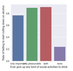
From the bivariate graph, we can see people who tend to give up both important and pleasurable activities to drink have the highest rate of failing to cut down on alcohol, which is around 90%, followed by the group who only give up pleasurable activities (88%) and only give up important activities (78%). People who are not giving up any social activities to drink has the lowest rate of failing to start cutting down on alcohol (22%). This shows that more social activities people are willing to give up for drinking, higher the chance of failing to cut down on alcohol.
Research question 2:
Association between “Failure of cutting down on alcohol” and “Severity of social relation damages”
“Severity of social relation damages” as response variable, and “More than once want to cut down on drinking” and “More than once unsuccessfully tried to cut down on alcohol” as dependent variables.
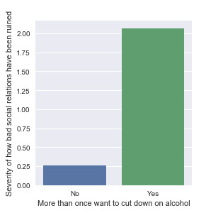
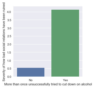
From the bivariate graphs, it is obvious to see that people who have struggles to cut down on drinking have ruined their social relations deeper than those who are not struggling. The y-axis represents the mean value of the severity of their affected social relations because of drinking. People who more than once want to cut down on drinking has an average value of 2.1 out of 10. And those who more than once unsuccessfully tried to cut down on drinking has their social relations damage severity score 4.1 out of 10. (Severity 0 to 10, higher the value, more damages caused) It also makes sense that people who have actually tried to cut down has a higher severity value than those who just want to. It is either the damaged relations make them feel obliged to quit drinking too much, or their struggling has make their relationship more difficult to be built back.
Research question 3:
Association between “age at onset of alcohol dependence” and “the number of episodes and the duration of the longest episode”
“the number of episodes and the duration of the longest episode” as response variable, and “age at onset of alcohol dependence” as dependent variables.
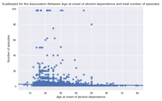
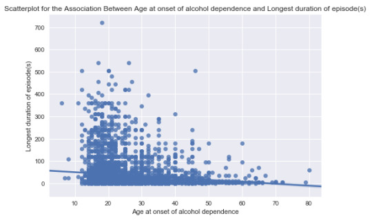
From the scatter plots, there seems to be no relations discovered between the selected variables. I think there might be more factors that affect the number and duration of the episodes. And the effect of how old to be onset of alcohol dependence could be neglected.
Research question 4:
Association between “fail to cut down on alcohol drinking” and “factors related to alcohol dependence”
“the age at onset of alcohol dependence, the number of episodes and the duration of the longest episode(s)” as response variable, and “rate of failing to cut down on alcohol” as dependent variables.
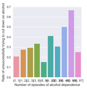
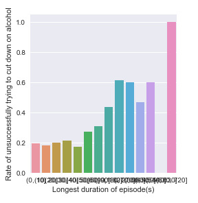
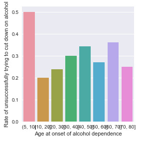
From the bar charts. I draw three conclusions:
1. People who are onset of alcohol dependence at very young age (from 5 years old to 10 years old) shows 50% of the chance of having difficulty in cutting down drinking.It may due to the fact that data sample is too small to be representative. And there is no obvious relation found in other age ranges.
2. People who have more times of alcohol dependence tend to face more difficulties in cutting down alcohol drinking. Because in general, we can see the rate increase as the number of episodes rise.
3. People who experienced longer duration of the episode of alcohol dependence tend to have more trouble of cutting down on alcohol. This also makes sense.
0 notes
Text
Assignment 3 Managing Data
From last assignment, I ran the first program that obtained the frequency distribution of the four variables mentioned in the main research question. For this week, I focus more on how to manage the data to approach the correlation between variables using the Technics taught. Following improvements were made in this week:
1. Code out missing data:
For most of the variables that I have chosen, their responses all include “unknown”. This is a response without valid information, therefore, I use function “replace” to code out all the responses that are “unknown”.

2. Add more variables and using data grouping techniques to simplify frequency distribution:
To further explore my research question, I found out there might also be a correlation between social relationship and alcohol dependence. So, I add three more variables related to the alcohol dependence:
These three variables involved age at onset of alcohol dependence and duration of episodes of alcohol dependence, and the values these variables take are many. Therefore, I use data grouping method to reduce the number of categories, which also simplify the frequency distribution without affecting data examination.
And here is how the output looks like:
3. Create secondary data and make more sense by recoding the value:
The first research question is that the more people participate social activities, more difficult it is to cut off on alcohol. And to explore more, I suspect not capable of cutting off on alcohol will also cause one’s social relations ruined. Therefore, four more variables are introduced:
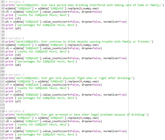
After coding out the missing data, here is the output of their frequency distribution:
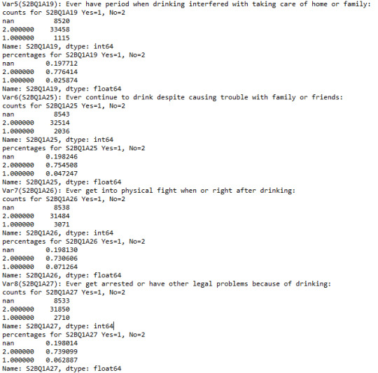
From here, it shows a trend of increasing severity of the issue in social relations. Starting from being less care, to causing trouble and having legal problem sue to drinking. Therefore, to make more sense of the variable, I decide to create a secondary variable based on these four variables. This secondary variable reveals how severe the social relations with families and friends have been ruined because of drinking.
This variable is called “SOCIALRUIN”. I rank the four issues from 1 point to 4 points based on their severity. Since the response “2” means no, and “1” means yes, I think it would be make more sense to recode “0” to all the negative response, instead of “2”. So, after I define the secondary variable as:
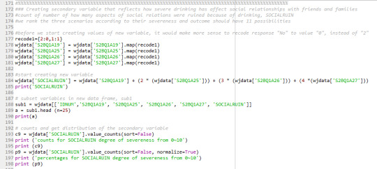
The value of “SOCIALRUIN” will take from 0 to 10. Higher the value, more damaged the one’s social relations have been. Here is frequency distribution of the secondary variable:
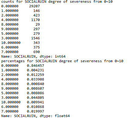
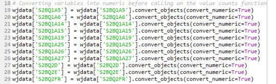
P.S. I have one problem with not being able to display the value by ascending order in the frequency distribution table. I know in the last week, there has been one program to solve this which is to convert the value into numeric. I have done this at the beginning, and I can see all the values become float type. However, they are not in order after distributed.
0 notes