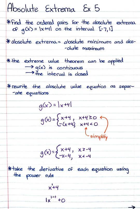
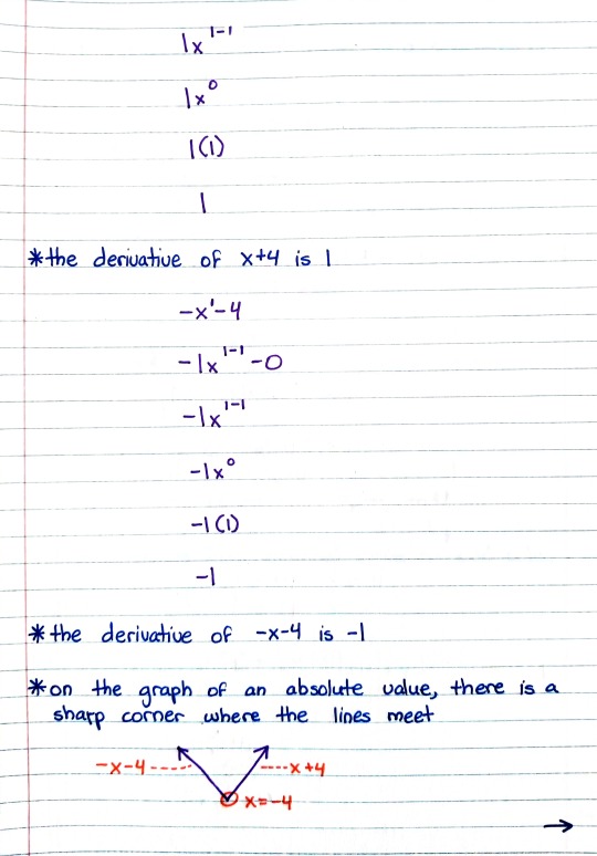
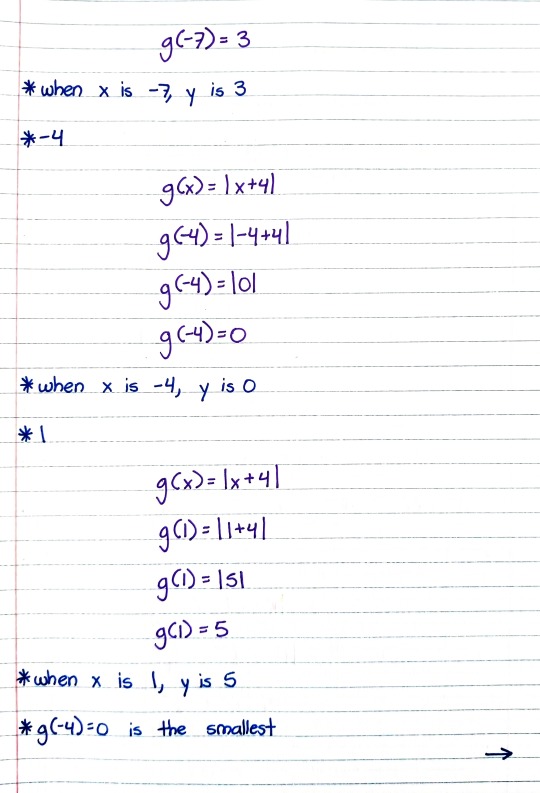
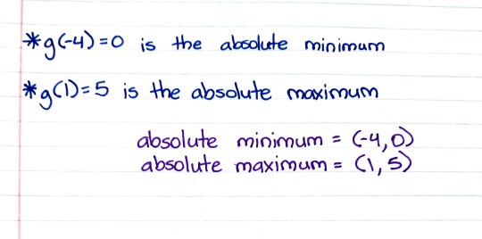
#absolute extrema example
Photo

Patreon | Ko-fi
#studyblr#notes#math#maths#mathblr#math notes#maths notes#absolute extrema#absolute extrema notes#absolute extrema ex#absolute extrema example#calculus#calculus notes#calculus ex#calculus example#calculus i#calculus 1#calculus 1 notes#calculus i notes
19 notes
·
View notes
Text
10.4 Usubstitution Trig Functionsap Calculus

10.4 U-substitution Trig Functionsap Calculus Answers
10.4 U-substitution Trig Functionsap Calculus Pdf
10.4 U-substitution Trig Functionsap Calculus Problems
10.4 U-substitution Trig Functionsap Calculus Worksheet
Calculus II, Section 7.4, #67 Integration of Rational Functions by Partial Fractions One method of slowing the growth of an insect population without the use of pesticides is to introduce into the population a number of sterile males that mate with fertile females but produce no o spring. Let P represeent. AP Calculus AB Mu Alpha Theta Welcome to AP Calculus AB! Contact me here. Need more review? Browse the Algebra II and Pre-Calculus Tabs. AP ® Calculus AB and BC. COURSE AND EXAM DESCRIPTION. AP COURSE AND EXAM DESCRIPTIONS ARE UPDATED PERIODICALLY. Please visit AP Central. Mathematics 104—Calculus, Part I (4h, 1 CU) Course Description: Brief review of High School Calculus, methods and applications of integration, infinite series, Taylor's theorem, first order ordinary differential equations. Use of symbolic manipulation and graphics software in Calculus. Note: This course uses Maple®.
Math 104: Calculus I – Notes
Section 004 - Spring 2014
10.4 U-substitution Trig Functionsap Calculus Answers
Syllabus
Concept Videos
Skeleton NotesComplete Notes
Title
More
Remainder 10.6, 10.9
Remainder 10.6/10.9
Series Estimation & Remainder
Sections 10.8-10.10
Sections 10.8-10.10
Taylor (and Maclaurin) Series
Section 10.7
Section 10.7
Power Series Introduction
Section 10.6
Section 10.6
Alt. Series Test and Abs. Conv.
Conv. Tests
Section 10.5
Section 10.5
The Ratio and Root Tests
Section 10.4
Section 10.4
The Comparison Tests
Section 10.3
Section 10.3
The Integral Test
Section 10.2
Section 10.2
Introduction to Series
Section 10.1
Section 10.1
Sequences
Section 9.2
Section 9.2
Linear Differential Equations
Section 7.2 Pt 1Pt 2
Section 7.2
Separable Differential Equations
Section 8.8
Section 8.8
Probability and Calculus
Odd Ans.
Section 8.7 Pt. 1Pt. 2Section 8.7
Improper Integrals
L'Hopital
Section 8.4 Pt. 1Pt. 2Section 8.4
Partial Fraction Decomposition
Section 8.3 Pt. 1Pt. 2Section 8.3
Trig. Substitution
Section 8.2 Pt. 1Pt. 2Section 8.2
Integrating Trig. Powers
Section 8.1 Pt. 1Pt. 2
Section 8.1
Integration By Parts
Section 6.6
Section 6.6
Center of Mass
Section 6.4
Section 6.4
Surface Area of Revolution
Section 6.3
Section 6.3
Arc Length
Section 6.2Section 6.2
Volumes Using Cylindrical Shells
Section 6.1
Section 6.1
Volumes Using Cross-Sections
disk/washer
Review
Calc I Review
Calc I ReviewLimit, Derivative, and Integral
Area b/w CurvesArea b/w Curves Video Example
U-substitution
Graphs you should know
Print out the skeleton notes before class and bring
them to class so that you don't have to write down
https://foxspain82.tumblr.com/post/657282647494672384/achievement-unlocked-2watermelon-gaming. Hide paragraph marks in microsoft word for mac. everything said in class. If you miss anything, the
complete notes will be posted after class.
10.4 U-substitution Trig Functionsap Calculus Pdf
My Penn Page | Penn Math 104 Page| Penn Undergraduate Math | Advice | Help|
10.4 U-substitution Trig Functionsap Calculus Problems
10.4 U-substitution Trig Functionsap Calculus Worksheet
Version #1
The course below follows CollegeBoard's Course and Exam Description. Lessons will begin to appear starting summer 2020.
BC Topics are listed, but there will be no lessons available for SY 2020-2021
Unit 0 - Calc Prerequisites (Summer Work)
0.1 Summer Packet
Unit 1 - Limits and Continuity
1.1 Can Change Occur at an Instant?
1.2 Defining Limits and Using Limit Notation
1.3 Estimating Limit Values from Graphs
1.4 Estimating Limit Values from Tables
1.5 Determining Limits Using Algebraic Properties
(1.5 includes piecewise functions involving limits)
1.6 Determining Limits Using Algebraic Manipulation
1.7 Selecting Procedures for Determining Limits
(1.7 includes rationalization, complex fractions, and absolute value)
1.8 Determining Limits Using the Squeeze Theorem
1.9 Connecting Multiple Representations of Limits
Mid-Unit Review - Unit 1
1.10 Exploring Types of Discontinuities
1.11 Defining Continuity at a Point
1.12 Confirming Continuity Over an Interval
1.13 Removing Discontinuities
1.14 Infinite Limits and Vertical Asymptotes
1.15 Limits at Infinity and Horizontal Asymptotes
1.16 Intermediate Value Theorem (IVT)
Review - Unit 1
Unit 2 - Differentiation: Definition and Fundamental Properties
2.1 Defining Average and Instantaneous Rate of
Change at a Point
2.2 Defining the Derivative of a Function and Using
Derivative Notation
(2.2 includes equation of the tangent line)
2.3 Estimating Derivatives of a Function at a Point
2.4 Connecting Differentiability and Continuity
2.5 Applying the Power Rule
2.6 Derivative Rules: Constant, Sum, Difference, and
Constant Multiple
(2.6 includes horizontal tangent lines, equation of the
normal line, and differentiability of piecewise)
2.7 Derivatives of cos(x), sin(x), e^x, and ln(x)
2.8 The Product Rule
2.9 The Quotient Rule
2.10 Derivatives of tan(x), cot(x), sec(x), and csc(x)
Review - Unit 2
Unit 3 - Differentiation: Composite, Implicit, and Inverse Functions
3.1 The Chain Rule
3.2 Implicit Differentiation
3.3 Differentiating Inverse Functions
3.4 Differentiating Inverse Trigonometric Functions
3.5 Selecting Procedures for Calculating Derivatives
3.6 Calculating Higher-Order Derivatives
Review - Unit 3
Unit 4 - Contextual Applications of Differentiation
4.1 Interpreting the Meaning of the Derivative in Context
4.2 Straight-Line Motion: Connecting Position, Velocity,
and Acceleration
4.3 Rates of Change in Applied Contexts Other Than
Motion
4.4 Introduction to Related Rates
4.5 Solving Related Rates Problems
4.6 Approximating Values of a Function Using Local
Linearity and Linearization
4.7 Using L'Hopital's Rule for Determining Limits of
Indeterminate Forms
Review - Unit 4
Unit 5 - Analytical Applications of Differentiation
5.1 Using the Mean Value Theorem
5.2 Extreme Value Theorem, Global Versus Local
Extrema, and Critical Points
5.3 Determining Intervals on Which a Function is
Increasing or Decreasing
5.4 Using the First Derivative Test to Determine Relative
Local Extrema
5.5 Using the Candidates Test to Determine Absolute
(Global) Extrema
5.6 Determining Concavity of Functions over Their
Domains
5.7 Using the Second Derivative Test to Determine
Extrema
Mid-Unit Review - Unit 5
5.8 Sketching Graphs of Functions and Their Derivatives
5.9 Connecting a Function, Its First Derivative, and Its
Second Derivative
(5.9 includes a revisit of particle motion and
determining if a particle is speeding up/down.)
5.10 Introduction to Optimization Problems
5.11 Solving Optimization Problems
5.12 Exploring Behaviors of Implicit Relations
Review - Unit 5
Unit 6 - Integration and Accumulation of Change
6.1 Exploring Accumulation of Change
6.2 Approximating Areas with Riemann Sums
6.3 Riemann Sums, Summation Notation, and Definite
Integral Notation
6.4 The Fundamental Theorem of Calculus and
Accumulation Functions
6.5 Interpreting the Behavior of Accumulation Functions
Involving Area
Mid-Unit Review - Unit 6
6.6 Applying Properties of Definite Integrals
6.7 The Fundamental Theorem of Calculus and Definite
Integrals
6.8 Finding Antiderivatives and Indefinite Integrals:
Basic Rules and Notation
6.9 Integrating Using Substitution
6.10 Integrating Functions Using Long Division
and Completing the Square
6.11 Integrating Using Integration by Parts (BC topic)
6.12 Integrating Using Linear Partial Fractions (BC topic)
6.13 Evaluating Improper Integrals (BC topic)
6.14 Selecting Techniques for Antidifferentiation
Review - Unit 6
Unit 7 - Differential Equations
7.1 Modeling Situations with Differential Equations
7.2 Verifying Solutions for Differential Equations
7.3 Sketching Slope Fields
7.4 Reasoning Using Slope Fields
7.5 Euler's Method (BC topic)
7.6 General Solutions Using Separation of Variables
7.7 Particular Solutions using Initial Conditions and
Separation of Variables
7.8 Exponential Models with Differential Equations
7.9 Logistic Models with Differential Equations (BC topic)
Review - Unit 7
Unit 8 - Applications of Integration
8.1 Average Value of a Function on an Interval
8.2 Position, Velocity, and Acceleration Using Integrals
8.3 Using Accumulation Functions and Definite Integrals
in Applied Contexts
8.4 Area Between Curves (with respect to x)
8.5 Area Between Curves (with respect to y)
8.6 Area Between Curves - More than Two Intersections
Mid-Unit Review - Unit 8
8.7 Cross Sections: Squares and Rectangles
8.8 Cross Sections: Triangles and Semicircles
8.9 Disc Method: Revolving Around the x- or y- Axis
8.10 Disc Method: Revolving Around Other Axes
8.11 Washer Method: Revolving Around the x- or y- Axis
8.12 Washer Method: Revolving Around Other Axes
8.13 The Arc Length of a Smooth, Planar Curve and
Distance Traveled (BC topic)
Review - Unit 8
Unit 9 - Parametric Equations, Polar Coordinates, and Vector-Valued Functions (BC topics)
9.1 Defining and Differentiating Parametric Equations
9.2 Second Derivatives of Parametric Equations
9.3 Arc Lengths of Curves (Parametric Equations)
9.4 Defining and Differentiating Vector-Valued Functions
9.5 Integrating Vector-Valued Functions
9.6 Solving Motion Problems Using Parametric and
Vector-Valued Functions
9.7 Defining Polar Coordinates and Differentiating in
Polar Form
9.8 Find the Area of a Polar Region or the Area Bounded
by a Single Polar Curve
9.9 Finding the Area of the Region Bounded by Two
Polar Curves
Review - Unit 9
Unit 10 - Infinite Sequences and Series (BC topics)
10.1 Defining Convergent and Divergent Infinite Series
10.2 Working with Geometric Series
10.3 The nth Term Test for Divergence
10.4 Integral Test for Convergence
10.5 Harmonic Series and p-Series
10.6 Comparison Tests for Convergence
10.7 Alternating Series Test for Convergence
10.8 Ratio Test for Convergence
10.9 Determining Absolute or Conditional Convergence
10.10 Alternating Series Error Bound
10.11 Finding Taylor Polynomial Approximations of
Functions
10.12 Lagrange Error Bound
10.13 Radius and Interval of Convergence of Power
Series
10.14 Finding Taylor Maclaurin Series for a Function
10.15 Representing Functions as a Power Series
Review - Unit 8
Version #2
The course below covers all topics for the AP Calculus AB exam, but was built for a 90-minute class that meets every other day.
Lessons and packets are longer because they cover more material.
Unit 0 - Calc Prerequisites (Summer Work)
0.1 Things to Know for Calc
0.2 Summer Packet
0.3 Calculator Skillz
Unit 1 - Limits
1.1 Limits Graphically
1.2 Limits Analytically
1.3 Asymptotes
1.4 Continuity
Review - Unit 1
Unit 2 - The Derivative
2.1 Average Rate of Change
2.2 Definition of the Derivative
2.3 Differentiability (Calculator Required)
Review - Unit 2
Unit 3 - Basic Differentiation
3.1 Power Rule
3.2 Product and Quotient Rules
3.3 Velocity and other Rates of Change
3.4 Chain Rule
3.5 Trig Derivatives
Review - Unit 3
Unit 4 - More Deriviatvies
4.1 Derivatives of Exp. and Logs
4.2 Inverse Trig Derivatives
4.3 L'Hopital's Rule
Review - Unit 4
Unit 5 - Curve Sketching
5.1 Extrema on an Interval
5.2 First Derivative Test
5.3 Second Derivative Test
Review - Unit 5
Unit 6 - Implicit Differentiation
6.1 Implicit Differentiation
6.2 Related Rates
6.3 Optimization
Review - Unit 6
Unit 7 - Approximation Methods
7.1 Rectangular Approximation Method
7.2 Trapezoidal Approximation Method
Review - Unit 7
Unit 8 - Integration
8.1 Definite Integral
8.2 Fundamental Theorem of Calculus (part 1)
8.3 Antiderivatives (and specific solutions)
Review - Unit 8
Unit 9 - The 2nd Fundamental Theorem of Calculus
9.1 The 2nd FTC
9.2 Trig Integrals
9.3 Average Value (of a function)
9.4 Net Change
Review - Unit 9
Unit 10 - More Integrals
10.1 Slope Fields
10.2 u-Substitution (indefinite integrals)
10.3 u-Substitution (definite integrals)
10.4 Separation of Variables
Review - Unit 10
Unit 11 - Area and Volume
11.1 Area Between Two Curves
11.2 Volume - Disc Method
11.3 Volume - Washer Method
11.4 Perpendicular Cross Sections
Review - Unit 11
0 notes
Text
Absolute Minimum

Free Minimum Calculator - find the Minimum of a data set step-by-step This website uses cookies to ensure you get the best experience. By using this website, you agree to our Cookie Policy. WordReference Random House Unabridged Dictionary of American English © 2019 ab′solute min′imumMath. Mathematics the smallest value a given function assumes on a specified set. ' absolute minimum ' also found in these entries. 👉 Learn how to determine the extrema from a graph. The extrema of a function are the critical points or the turning points of the function. They are the poi.
Absolute Minimum Math
Show Mobile NoticeShow All NotesHide All Notes

You appear to be on a device with a 'narrow' screen width (i.e. you are probably on a mobile phone). Due to the nature of the mathematics on this site it is best views in landscape mode. If your device is not in landscape mode many of the equations will run off the side of your device (should be able to scroll to see them) and some of the menu items will be cut off due to the narrow screen width.
Section 4-3 : Minimum and Maximum Values
Many of our applications in this chapter will revolve around minimum and maximum values of a function. While we can all visualize the minimum and maximum values of a function we want to be a little more specific in our work here. In particular, we want to differentiate between two types of minimum or maximum values. The following definition gives the types of minimums and/or maximums values that we’ll be looking at.
Definition
We say that (fleft( x right)) has an absolute (or global) maximum at (x = c) if(fleft( x right) le fleft( c right)) for every (x) in the domain we are working on.
We say that (fleft( x right)) has a relative (or local) maximum at (x = c) if (fleft( x right) le fleft( c right)) for every (x) in some open interval around (x = c).
We say that (fleft( x right)) has an absolute (or global) minimum at (x = c) if (fleft( x right) ge fleft( c right)) for every (x) in the domain we are working on.
We say that (fleft( x right)) has a relative (or local) minimum at (x = c) if(fleft( x right) ge fleft( c right)) for every (x) in some open interval around (x = c).
Note that when we say an “open interval around(x = c)” we mean that we can find some interval (left( {a,b} right)), not including the endpoints, such that (a < c < b). Or, in other words, (c) will be contained somewhere inside the interval and will not be either of the endpoints.
Also, we will collectively call the minimum and maximum points of a function the extrema of the function. So, relative extrema will refer to the relative minimums and maximums while absolute extrema refer to the absolute minimums and maximums.
Now, let’s talk a little bit about the subtle difference between the absolute and relative in the definition above.
We will have an absolute maximum (or minimum) at (x = c) provided (fleft( c right)) is the largest (or smallest) value that the function will ever take on the domain that we are working on. Also, when we say the “domain we are working on” this simply means the range of (x)’s that we have chosen to work with for a given problem. There may be other values of (x) that we can actually plug into the function but have excluded them for some reason.
A relative maximum or minimum is slightly different. All that’s required for a point to be a relative maximum or minimum is for that point to be a maximum or minimum in some interval of (x)’s around (x = c). There may be larger or smaller values of the function at some other place, but relative to (x = c), or local to (x = c), (fleft( c right)) is larger or smaller than all the other function values that are near it.
Note as well that in order for a point to be a relative extrema we must be able to look at function values on both sides of (x = c) to see if it really is a maximum or minimum at that point. This means that relative extrema do not occur at the end points of a domain. They can only occur interior to the domain.
There is actually some debate on the preceding point. Some folks do feel that relative extrema can occur on the end points of a domain. However, in this class we will be using the definition that says that they can’t occur at the end points of a domain. This will be discussed in a little more detail at the end of the section once we have a relevant fact taken care of.
It’s usually easier to get a feel for the definitions by taking a quick look at a graph.
For the function shown in this graph we have relative maximums at (x = b) and (x = d). Both of these points are relative maximums since they are interior to the domain shown and are the largest point on the graph in some interval around the point. We also have a relative minimum at (x = c) since this point is interior to the domain and is the lowest point on the graph in an interval around it. The far-right end point, (x = e), will not be a relative minimum since it is an end point.
The function will have an absolute maximum at (x = d) and an absolute minimum at (x = a). These two points are the largest and smallest that the function will ever be. We can also notice that the absolute extrema for a function will occur at either the endpoints of the domain or at relative extrema. We will use this idea in later sections so it’s more important than it might seem at the present time.
Let’s take a quick look at some examples to make sure that we have the definitions of absolute extrema and relative extrema straight.
Example 1 Identify the absolute extrema and relative extrema for the following function. [fleft( x right) = {x^2}hspace{0.25in}{mbox{on}}hspace{0.25in}left[ { - 1,2} right]] Show Solution
Since this function is easy enough to graph let’s do that. However, we only want the graph on the interval (left[ { - 1,2} right]). Here is the graph,
Note that we used dots at the end of the graph to remind us that the graph ends at these points.
We can now identify the extrema from the graph. It looks like we’ve got a relative and absolute minimum of zero at (x = 0) and an absolute maximum of four at (x = 2). Note that (x = - 1) is not a relative maximum since it is at the end point of the interval.
This function doesn’t have any relative maximums.
As we saw in the previous example functions do not have to have relative extrema. It is completely possible for a function to not have a relative maximum and/or a relative minimum.
Example 2 Identify the absolute extrema and relative extrema for the following function. [fleft( x right) = {x^2}hspace{0.25in}{mbox{on}}hspace{0.25in}left[ { - 2,2} right]] Show Solution
Here is the graph for this function.
In this case we still have a relative and absolute minimum of zero at (x = 0). We also still have an absolute maximum of four. However, unlike the first example this will occur at two points, (x = - 2) and (x = 2).
Again, the function doesn’t have any relative maximums.
As this example has shown there can only be a single absolute maximum or absolute minimum value, but they can occur at more than one place in the domain.
Example 3 Identify the absolute extrema and relative extrema for the following function. [fleft( x right) = {x^2}] Show Solution
In this case we’ve given no domain and so the assumption is that we will take the largest possible domain. For this function that means all the real numbers. Here is the graph.
In this case the graph doesn’t stop increasing at either end and so there are no maximums of any kind for this function. No matter which point we pick on the graph there will be points both larger and smaller than it on either side so we can’t have any maximums (of any kind, relative or absolute) in a graph.
We still have a relative and absolute minimum value of zero at (x = 0).
So, some graphs can have minimums but not maximums. Likewise, a graph could have maximums but not minimums.
Example 4 Identify the absolute extrema and relative extrema for the following function. [fleft( x right) = {x^3}hspace{0.25in}{mbox{on}}hspace{0.25in}left[ { - 2,2} right]] Show Solution
Here is the graph for this function.
This function has an absolute maximum of eight at (x = 2) and an absolute minimum of negative eight at (x = - 2). This function has no relative extrema.
So, a function doesn’t have to have relative extrema as this example has shown.
Example 5 Identify the absolute extrema and relative extrema for the following function. [fleft( x right) = {x^3}] Show Solution
Again, we aren’t restricting the domain this time so here’s the graph.
In this case the function has no relative extrema and no absolute extrema.
As we’ve seen in the previous example functions don’t have to have any kind of extrema, relative or absolute.
Example 6 Identify the absolute extrema and relative extrema for the following function. [fleft( x right) = cos left( x right)] Show Solution
We’ve not restricted the domain for this function. Here is the graph.
Cosine has extrema (relative and absolute) that occur at many points. Cosine has both relative and absolute maximums of 1 at
[x = ldots - 4pi , - 2pi ,0,2pi ,4pi , ldots ]
Cosine also has both relative and absolute minimums of -1 at
[x = ldots - 3pi , - pi ,pi ,3pi , ldots ]
As this example has shown a graph can in fact have extrema occurring at a large number (infinite in this case) of points.
We’ve now worked quite a few examples and we can use these examples to see a nice fact about absolute extrema. First let’s notice that all the functions above were continuous functions. Next notice that every time we restricted the domain to a closed interval (i.e. the interval contains its end points) we got absolute maximums and absolute minimums. Finally, in only one of the three examples in which we did not restrict the domain did we get both an absolute maximum and an absolute minimum.
These observations lead us the following theorem.
Extreme Value Theorem
Suppose that (fleft( x right)) is continuous on the interval (left[ {a,b} right]) then there are two numbers (a le c,d le b) so that (fleft( c right)) is an absolute maximum for the function and (fleft( d right)) is an absolute minimum for the function.
So, if we have a continuous function on an interval (left[ {a,b} right]) then we are guaranteed to have both an absolute maximum and an absolute minimum for the function somewhere in the interval. The theorem doesn’t tell us where they will occur or if they will occur more than once, but at least it tells us that they do exist somewhere. Sometimes, all that we need to know is that they do exist.
This theorem doesn’t say anything about absolute extrema if we aren’t working on an interval. We saw examples of functions above that had both absolute extrema, one absolute extrema, and no absolute extrema when we didn’t restrict ourselves down to an interval.
The requirement that a function be continuous is also required in order for us to use the theorem. Consider the case of
[fleft( x right) = frac{1}{{{x^2}}}hspace{0.25in}{mbox{on}}hspace{0.25in}[ - 1,1]]
Here’s the graph.
This function is not continuous at (x = 0) as we move in towards zero the function is approaching infinity. So, the function does not have an absolute maximum. Note that it does have an absolute minimum however. In fact the absolute minimum occurs twice at both (x = - 1) and (x = 1).
If we changed the interval a little to say,
[fleft( x right) = frac{1}{{{x^2}}}hspace{0.25in}{mbox{on}}hspace{0.25in}left[ {frac{1}{2},1} right]]
the function would now have both absolute extrema. We may only run into problems if the interval contains the point of discontinuity. If it doesn’t then the theorem will hold.
We should also point out that just because a function is not continuous at a point that doesn’t mean that it won’t have both absolute extrema in an interval that contains that point. Below is the graph of a function that is not continuous at a point in the given interval and yet has both absolute extrema.
This graph is not continuous at (x = c), yet it does have both an absolute maximum ((x = b)) and an absolute minimum ((x = c)). Also note that, in this case one of the absolute extrema occurred at the point of discontinuity, but it doesn’t need to. The absolute minimum could just have easily been at the other end point or at some other point interior to the region. The point here is that this graph is not continuous and yet does have both absolute extrema
The point of all this is that we need to be careful to only use the Extreme Value Theorem when the conditions of the theorem are met and not misinterpret the results if the conditions aren’t met.
In order to use the Extreme Value Theorem we must have an interval that includes its endpoints, often called a closed interval, and the function must be continuous on that interval. If we don’t have a closed interval and/or the function isn’t continuous on the interval then the function may or may not have absolute extrema.
We need to discuss one final topic in this section before moving on to the first major application of the derivative that we’re going to be looking at in this chapter.
Fermat’s Theorem
If (fleft( x right)) has a relative extrema at (x = c) and (f'left( c right)) exists then (x = c) is a critical point of (fleft( x right)). In fact, it will be a critical point such that (f'left( c right) = 0).
To see the proof of this theorem see the Proofs From Derivative Applications section of the Extras chapter.
Also note that we can say that (f'left( c right) = 0) because we are also assuming that (f'left( c right)) exists.
This theorem tells us that there is a nice relationship between relative extrema and critical points. In fact, it will allow us to get a list of all possible relative extrema. Since a relative extrema must be a critical point the list of all critical points will give us a list of all possible relative extrema.
Consider the case of (fleft( x right) = {x^2}). We saw that this function had a relative minimum at (x = 0) in several earlier examples. So according to Fermat’s theorem (x = 0) should be a critical point. The derivative of the function is,
[f'left( x right) = 2x]
Sure enough (x = 0) is a critical point.
Be careful not to misuse this theorem. It doesn’t say that a critical point will be a relative extrema. To see this, consider the following case.
[fleft( x right) = {x^3}hspace{0.25in}hspace{0.25in}f'left( x right) = 3{x^2}]
Clearly (x = 0) is a critical point. However, we saw in an earlier example this function has no relative extrema of any kind. So, critical points do not have to be relative extrema.
Also note that this theorem says nothing about absolute extrema. An absolute extrema may or may not be a critical point.
Before we leave this section we need to discuss a couple of issues.
First, Fermat’s Theorem only works for critical points in which (f'left( c right) = 0). This does not, however, mean that relative extrema won’t occur at critical points where the derivative does not exist. To see this consider (fleft( x right) = left| x right|). This function clearly has a relative minimum at (x = 0) and yet in a previous section we showed in an example that (f'left( 0 right)) does not exist.
What this all means is that if we want to locate relative extrema all we really need to do is look at the critical points as those are the places where relative extrema may exist.
Absolute Minimum Math
Finally, recall that at that start of the section we stated that relative extrema will not exist at endpoints of the interval we are looking at. The reason for this is that if we allowed relative extrema to occur there it may well (and in fact most of the time) violate Fermat’s Theorem. There is no reason to expect end points of intervals to be critical points of any kind. Therefore, we do not allow relative extrema to exist at the endpoints of intervals.
0 notes
Text

EXTREMA OF FUNCTIONS
Hi! It's been a month since my last post. We are down to the last quarter of this school year!! For this week, we will be discussing Extrema of Functions. Let's check the examples below:
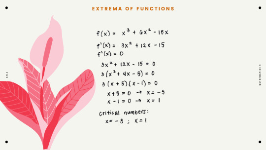
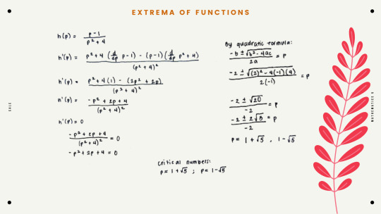
For the examples above, we are tasked to find the critical numbers for each function. The definition of critical number is: a number c in the domain of f such that either f'(c)=0 or f'(c) does not exist. This is why the first derivative of the functions above were equated to 0 to find the critical numbers. We also need to make sure that the numbers solved are in the domain of f to consider them as the critical numbers of the function.


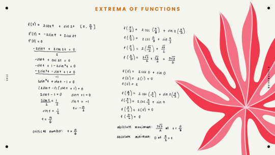
In the examples above, we are tasked to find the absolute maximum and the absolute minimum values of f in the given intervals. First, we need to find the critical numbers of the functions. Then we will use the Closed Interval Method to find the absolute minimum and maximum values. This is done by finding the value of f at the critical number(s) and at the endpoints of the interval. The largest value is the absolute maximum while the smallest value is the absolute minimum.
Reflection (Week 1)

My mind still can't process that we are now at the last quarter of the school year. I think this is why during this week, I did not do much in this subject. I did not study the learning guides right away. I just started after the synchronous class, where we discussed the topic. I think this has been my habit since the second quarter which needs to be improved. I need to be more productive in the following weeks so that I won't have many backlogs, especially since our long test is scheduled next week. I also watched the supplementary videos which made my understanding of the topic better. I will my best to devote enough time for this subject. <3
1 note
·
View note
Text
herramienta albañil

Cuidados de la Poinsettia
En las fechas en las que estamos y con la Navidad rodeándonos por todos lados, es inevitable no pensar en la planta por excelencia de estas fiestas, la Poinsettia o Flor de Pascua.
Su vibrante color rojo decora casas, establecimientos, escaparates y calles otorgando elegancia y espíritu navideño como ninguna otra, ¡a nosotros nos encanta! Por eso no podíamos dejar pasar la oportunidad de dedicarle un post en el blog de Showroom Barral ahora que es su época.
DATOS Y CURIOSIDADES DE LA POINSETTIA
Es originaria de México y su nombre científico es Euphorbia pulcherrima. Popularmente es conocida por todo el mundo con diversos nombres como: Flor de Pascua, pascuero, Flor de Navidad, Flor de Nochebuena, Estrella de Navidad o Poinsettia.
El día 12 de diciembre se celebra el día Mundial de la Poinsettia en honor de J.R. Poinsett, que fue el primer embajador estadounidense en México. Introdujo la planta en Estados Unidos en 1825 y falleció en el año 1851 de este día.
El color rojo que vemos no son sus flores, son hojas y se llaman brácteas. Las flores son minúsculas y amarillas. Y aunque la variedad más conocida es la roja, existen más de 100 distintas. La Poinsettia de hojas rojas es la que más se comercializa, pero actualmente ya podemos encontrar a la venta también las variedades de hojas blancas, rosas o amarillas.
En España, el 25% de la producción está en Almería, más de 2 millones y medio de unidades. Sin duda tiene que ser toda una experiencia visual ver tantos ejemplares juntos rebosantes de color.
CUIDADOS DE LA POINSETTIA
Riego
No busques la regadera, porque la Flor de Pascua y ella no se llevan nada bien. Evita completamente rociar agua por encima de sus hojas.
Lo ideal es poner agua en el plato, dejar que la planta absorba lo que necesite (dar un margen de tiempo de aproximadamente 30 minutos), y después retirar del plato el agua que haya sobrado.
Con dos riegos a la semana bastaría, un exceso de agua pudriría rápidamente sus raíces.
Un buen truco, además, es dejar reposar el agua unas 24 horas antes de usarla para regar. Pues el agua del grifo o embotellada que usamos, lleva un proceso de potabilización en el que influye el cloro, y con el reposo se consigue su evaporación.
Luz y temperatura
Como casi todas las plantas de interior necesita luz, pero no directamente, para impedir que sus hojas se quemen. Lo idóneo es colocarla cerca de una ventana por la que entre luz, pero sin sol directo, y alejarla de fuentes de calor como radiadores, estufas…
Si observamos que las hojas más inferiores comienzan a caerse significa que le falta luz.
La Poinsettia es muy sensible a los cambios de temperatura, y no admite temperaturas muy extremas, ni de calor ni de frío. El margen perfecto al que debe encontrarse el ambiente es entre 12 y 24 grados centígrados. Este es uno de los aspectos más importantes de los cuidados de la Poinsettia.
Abono
Los meses centrales de crecimiento de la Flor de Pascua es de noviembre a enero, cuando las noches son más largas que los días.
En estos meses es ideal utilizar abonos, ya sean líquidos, compactos o granulados, para ayudar a nuestra Poinsettia a no perder su color rojo, a que crezcan más hojas y a potenciar su desarrollo.
La forma y tiempo de administración del abono escogido deberemos realizarlo según las instrucciones del fabricante.
Trasplante
Si pasadas las fechas navideñas nuestra Poinsettia continúa en perfectas condiciones y queremos alargar su vida, lo ideal es dejarla en la misma maceta hasta los meses de marzo o abril, cuando las condiciones climatológicas cambian.
Es entonces cuando podemos trasplantarla a una maceta más grande, podar sus ramas y renovar el sustrato. Podemos también colocarla en el exterior (recuerda, sin sol directo), ya que las temperaturas son idóneas.
En estos meses el color rojizo (u otro según la variedad) desaparecerá, y solo veremos las hojas verdes. Pero si conseguimos mantenerla en un buen ambiente y con los cuidados necesarios durante el verano y otoño, al llegar de nuevo noviembre comenzarán de nuevo a teñirse de color sus brácteas.
Esperamos que con estas indicaciones y tus cuidados consigas mantener tu Poinsettia o Flor de Pascua todo el tiempo que desees. En Showroom Barral nos encanta la naturaleza, y el cuidado de las plantas es un trabajo muy bello y gratificante.
No dudes en consultar nuestra sección de jardín para buscar todo lo que necesites, y en consultar con nuestros profesionales si tienes alguna duda, ¡te esperamos!
Fine-tune heating systems
The drop in temperatures has been noted and the arrival of winter is approaching. Probably - depending on the area of Spain in which you reside - you are already thinking about turning on the heating or even if you have already done so, these tips may arrive on time and be useful to you.
Setting up the heating systems of our home is essential not only to avoid wasting the energy and heat they provide, but also to prevent breakdowns in appliances and possible more serious accidents in our home.
Whichever heating system is used, an overhaul is absolutely necessary before starting it up. Either ourselves checking some basic aspects, or by a specialized technician, as is the case with boilers.
Next, from Showroom Barral we summarize the steps and essential aspects that must be taken into account to fine-tune the different heating systems. Remember that if there is a step that you are not sure how to carry out, it is better that you contact a professional to avoid accidents.
Gas or diesel boilers
The most important thing is to keep the pressure at the appropriate values, which is between 1.2 and 1.5 bar (unit of pressure measurement). All boilers have a pressure gauge to see the pressure, or in the most modern, a digital display.
If the pressure is below or above the recommended values, take the instruction manual of your boiler to know how to adjust it correctly. A pressure with inappropriate values can have negative effects on our boiler and cause a serious failure.
In addition, it is advisable to take a look around the visible circuit to check that there are no water leaks or a badly connected cable or conduit. In case of finding any type of leak or fault, it is time to contact the specialist.
For both types of boilers an annual review is usually carried out by the technician. In addition to gas, the distribution company must carry out a mandatory review every two or five years, depending on its characteristics.
Radiators
Bleed and radiators always go hand in hand. Purging is simply removing the air that is inside the radiator, after several months without working it is normal for air to “leak”.
The fact that radiators store air inside may cause the radiator to not heat evenly. For example, that the upper part is cold or barely warm and as we lower our hand we notice that it is very hot; or we may hear strange noises, such as "gurgling" when turning on the heater.
To bleed the radiators make sure first that the heating is off. Then follow the order from the one closest to the boiler to the one furthest away. Locate where the drain cock is and place a container under it so as not to stain the floor. Simply use a coin or screwdriver to turn the valve and you will notice how water and air begin to come out discontinuously. Once only water comes out it means that there is no more air left, so you can close the valve and continue with the next radiator.
Air conditioning with heat pump
As during its use in summer in cold mode, in heat pump air conditioners it is important to clean the air filters periodically to ensure proper operation and optimal air quality.
Pellet stoves or biomass stoves
In recent years this type of heating system has been in high demand since pellet stoves provide great calorific power and good performance and also do so with renewable energy, which is why they are more ecological than the gas or oil boilers mentioned above. .
Its maintenance, however, requires more dedication. An annual review by the expert technician, and daily / weekly care is recommended. Such as cleaning the ashtray, so that the ashes do not clog the ducts, and cleaning the combustion chamber.
Gas stoves and electric heaters
They are more traditional methods of calorific contribution. Today they are not usually found as the main method of heating the home, but they are in specific rooms or for specific moments. They need some prior considerations to avoid serious domestic accidents.
In the case of gas stoves, also known as catalytic stoves, it is vitally important to check the good condition of the rubber that connects the stove to the cylinder, as well as its expiration date.
On the other hand, in electric heaters it is necessary to check that the connection cable is in good condition and clean the resistors to remove the accumulation of dust or other particles.
Contact Us
Address: - HB Barral Avenida de la Cañada, 4628823 Coslada Madrid Spain
Phone: - 673 53 96 63
Email: - [email protected]
More Information: - Barral.com
0 notes
Text
tienda de materiales de construccion

Cuidados de la Poinsettia
En las fechas en las que estamos y con la Navidad rodeándonos por todos lados, es inevitable no pensar en la planta por excelencia de estas fiestas, la Poinsettia o Flor de Pascua.
Su vibrante color rojo decora casas, establecimientos, escaparates y calles otorgando elegancia y espíritu navideño como ninguna otra, ¡a nosotros nos encanta! Por eso no podíamos dejar pasar la oportunidad de dedicarle un post en el blog de Showroom Barral ahora que es su época.
DATOS Y CURIOSIDADES DE LA POINSETTIA
Es originaria de México y su nombre científico es Euphorbia pulcherrima. Popularmente es conocida por todo el mundo con diversos nombres como: Flor de Pascua, pascuero, Flor de Navidad, Flor de Nochebuena, Estrella de Navidad o Poinsettia.
El día 12 de diciembre se celebra el día Mundial de la Poinsettia en honor de J.R. Poinsett, que fue el primer embajador estadounidense en México. Introdujo la planta en Estados Unidos en 1825 y falleció en el año 1851 de este día.
El color rojo que vemos no son sus flores, son hojas y se llaman brácteas. Las flores son minúsculas y amarillas. Y aunque la variedad más conocida es la roja, existen más de 100 distintas. La Poinsettia de hojas rojas es la que más se comercializa, pero actualmente ya podemos encontrar a la venta también las variedades de hojas blancas, rosas o amarillas.
En España, el 25% de la producción está en Almería, más de 2 millones y medio de unidades. Sin duda tiene que ser toda una experiencia visual ver tantos ejemplares juntos rebosantes de color.
CUIDADOS DE LA POINSETTIA
Riego
No busques la regadera, porque la Flor de Pascua y ella no se llevan nada bien. Evita completamente rociar agua por encima de sus hojas.
Lo ideal es poner agua en el plato, dejar que la planta absorba lo que necesite (dar un margen de tiempo de aproximadamente 30 minutos), y después retirar del plato el agua que haya sobrado.
Con dos riegos a la semana bastaría, un exceso de agua pudriría rápidamente sus raíces.
Un buen truco, además, es dejar reposar el agua unas 24 horas antes de usarla para regar. Pues el agua del grifo o embotellada que usamos, lleva un proceso de potabilización en el que influye el cloro, y con el reposo se consigue su evaporación.
Luz y temperatura
Como casi todas las plantas de interior necesita luz, pero no directamente, para impedir que sus hojas se quemen. Lo idóneo es colocarla cerca de una ventana por la que entre luz, pero sin sol directo, y alejarla de fuentes de calor como radiadores, estufas…
Si observamos que las hojas más inferiores comienzan a caerse significa que le falta luz.
La Poinsettia es muy sensible a los cambios de temperatura, y no admite temperaturas muy extremas, ni de calor ni de frío. El margen perfecto al que debe encontrarse el ambiente es entre 12 y 24 grados centígrados. Este es uno de los aspectos más importantes de los cuidados de la Poinsettia.
Abono
Los meses centrales de crecimiento de la Flor de Pascua es de noviembre a enero, cuando las noches son más largas que los días.
En estos meses es ideal utilizar abonos, ya sean líquidos, compactos o granulados, para ayudar a nuestra Poinsettia a no perder su color rojo, a que crezcan más hojas y a potenciar su desarrollo.
La forma y tiempo de administración del abono escogido deberemos realizarlo según las instrucciones del fabricante.
Trasplante
Si pasadas las fechas navideñas nuestra Poinsettia continúa en perfectas condiciones y queremos alargar su vida, lo ideal es dejarla en la misma maceta hasta los meses de marzo o abril, cuando las condiciones climatológicas cambian.
Es entonces cuando podemos trasplantarla a una maceta más grande, podar sus ramas y renovar el sustrato. Podemos también colocarla en el exterior (recuerda, sin sol directo), ya que las temperaturas son idóneas.
En estos meses el color rojizo (u otro según la variedad) desaparecerá, y solo veremos las hojas verdes. Pero si conseguimos mantenerla en un buen ambiente y con los cuidados necesarios durante el verano y otoño, al llegar de nuevo noviembre comenzarán de nuevo a teñirse de color sus brácteas.
Esperamos que con estas indicaciones y tus cuidados consigas mantener tu Poinsettia o Flor de Pascua todo el tiempo que desees. En Showroom Barral nos encanta la naturaleza, y el cuidado de las plantas es un trabajo muy bello y gratificante.
No dudes en consultar nuestra sección de jardín para buscar todo lo que necesites, y en consultar con nuestros profesionales si tienes alguna duda, ¡te esperamos!
Fine-tune heating systems
The drop in temperatures has been noted and the arrival of winter is approaching. Probably - depending on the area of Spain in which you reside - you are already thinking about turning on the heating or even if you have already done so, these tips may arrive on time and be useful to you.
Setting up the heating systems of our home is essential not only to avoid wasting the energy and heat they provide, but also to prevent breakdowns in appliances and possible more serious accidents in our home.
Whichever heating system is used, an overhaul is absolutely necessary before starting it up. Either ourselves checking some basic aspects, or by a specialized technician, as is the case with boilers.
Next, from Showroom Barral we summarize the steps and essential aspects that must be taken into account to fine-tune the different heating systems. Remember that if there is a step that you are not sure how to carry out, it is better that you contact a professional to avoid accidents.
Gas or diesel boilers
The most important thing is to keep the pressure at the appropriate values, which is between 1.2 and 1.5 bar (unit of pressure measurement). All boilers have a pressure gauge to see the pressure, or in the most modern, a digital display.
If the pressure is below or above the recommended values, take the instruction manual of your boiler to know how to adjust it correctly. A pressure with inappropriate values can have negative effects on our boiler and cause a serious failure.
In addition, it is advisable to take a look around the visible circuit to check that there are no water leaks or a badly connected cable or conduit. In case of finding any type of leak or fault, it is time to contact the specialist.
For both types of boilers an annual review is usually carried out by the technician. In addition to gas, the distribution company must carry out a mandatory review every two or five years, depending on its characteristics.
Radiators
Bleed and radiators always go hand in hand. Purging is simply removing the air that is inside the radiator, after several months without working it is normal for air to “leak”.
The fact that radiators store air inside may cause the radiator to not heat evenly. For example, that the upper part is cold or barely warm and as we lower our hand we notice that it is very hot; or we may hear strange noises, such as "gurgling" when turning on the heater.
To bleed the radiators make sure first that the heating is off. Then follow the order from the one closest to the boiler to the one furthest away. Locate where the drain cock is and place a container under it so as not to stain the floor. Simply use a coin or screwdriver to turn the valve and you will notice how water and air begin to come out discontinuously. Once only water comes out it means that there is no more air left, so you can close the valve and continue with the next radiator.
Air conditioning with heat pump
As during its use in summer in cold mode, in heat pump air conditioners it is important to clean the air filters periodically to ensure proper operation and optimal air quality.
Pellet stoves or biomass stoves
In recent years this type of heating system has been in high demand since pellet stoves provide great calorific power and good performance and also do so with renewable energy, which is why they are more ecological than the gas or oil boilers mentioned above. .
Its maintenance, however, requires more dedication. An annual review by the expert technician, and daily / weekly care is recommended. Such as cleaning the ashtray, so that the ashes do not clog the ducts, and cleaning the combustion chamber.
Gas stoves and electric heaters
They are more traditional methods of calorific contribution. Today they are not usually found as the main method of heating the home, but they are in specific rooms or for specific moments. They need some prior considerations to avoid serious domestic accidents.
In the case of gas stoves, also known as catalytic stoves, it is vitally important to check the good condition of the rubber that connects the stove to the cylinder, as well as its expiration date.
On the other hand, in electric heaters it is necessary to check that the connection cable is in good condition and clean the resistors to remove the accumulation of dust or other particles.
Contact Us
Address: - HB Barral Avenida de la Cañada, 4628823 Coslada Madrid Spain
Phone: - 673 53 96 63
Email: - [email protected]
More Information: - Barral.com
0 notes
Text
Variations of Annual Turnover Cycles for Nutrients in the North Sea, German Bight Nutrients Turnover Cycles in The North Sea- Juniper Publishers
Abstract
The long term behavior of water chemical composition in the North Sea, German Bight is much influenced by the atmospheric, hydrographical as well as biological processes. We analyze the long term trends in annual turnover cycles of the silicate, phosphate, nitrate and nitrite for the period of 1966-2009. We provide a straightforward numerical procedure for determination of the nutrients depletion phases.
It uses the rates of cumulative concentrations to distinguish among different phases of nutrients cycle. The silicate is one of the key nutrients used by diatoms. The amount of silicate also depends on the mixing of coastal and more marine water at Helgoland. We show that seasonal dynamics of silicate undergone a strong change since 1987 until 2009. It is characterized by an earlier onset of nutrients depletion and build-up phases. Also a shortening of nutrient depletion phases for both silicate and phosphate is observed during period 1966-1984/1985 For phosphate the start of depletion and build-up phases generally evolves towards later time of the year in the interval 1984-2009. Among other nutrients nitrate exhibits higher interannual and interseasonal variability over the whole time analyzed. The depletion cycle length for most of the nutrients (with exception of silicate) is negatively correlated with total annual concentrations. The annual sunshine hours are qualitatively compared with the onset and termination of depletion for phosphate and a good match between the variation of depletion phase and annual sunshine is observed.
Keywords: Nutrients cycles; Depletion rates; Silicate concentration; Long-term data; Nutrients limitation
Go to
Introduction
Wide-scale shifts in biological and abiotic variables has been reported to occur for the North and Wadden Sea in 1979, 1988 and 1998 [1]. In line with these results other studies report on large scale changes in various levels of ecosystem that took place in the late 1970s and 1980s [2-4].
The coastal region of the North Sea is characterized by the seasonal fluctuations of the climate and environmental conditions and biological population variability. This happens to the large extend due to the interplay between different water bodies: low salinity coastal and offshore marine waters. In addition coastal area is mainly driven by the atmospheric forcing and therefore is more sensitive to the climate change [5]. The ecosystem along the coast is largely affected by the local influence of increased nutrients concentrations [6]. Also the GB ecosystem is heavily impacted by anthropogenic perturbations.
Although numerous observations and statistical analysis of long term data support the clear evidence of the regime shifts in hydrographical, atmospheric and physicochemical variables [7] it remains unclear how these changes affect the base of marine food webs. And more general, is the coastal ecosystem affected by the wide-scale climate variations, can it be placed in the framework of the overall pattern on climate-ocean variability observed for the North Sea. For example, in spite of the fact that most of the parameters indicating water climate altered markedly no significant change of timing of seasonal diatom blooms at Helgoland has occur in years 1975-2005 [8]. At the same time analysis of phytoplankton species diversity and algal density shows a marked increase in the number of large diatoms [8]. The average cell size has increased from 0.1ng to 1-2ng. As a consequence of the increased percentage of large diatom cells the rate of primary production and resource reduction will be altered as well. The increase of numbers of cells with hard silicate shell introduces higher silicates demand in the ecosystem that it was found during previous period. To our knowledge the effects of increase of the cell sizes on the annual pattern of silicate turnover has not been studied so far. From the other hand there is a pronounced upward shift in silicate concentrations observed in late 1970s at HR.
Many long-term studies in the coastal North and Wadden Sea region highlight the importance of nutrients and water chemical composition on the local ecosystem developments [9]. In the GB the increase of biodiversity in mid 1990s of phyto-and zooplankton documented at Helgoland [8] by no means influences the routes of energy and nutrients transfer in the marine food web. One of the topics of interest is to investigate how the incline of percentage of large size diatoms [8] contributes to the change of nutrient depletion rates. In this paper we analyze the long-term trends in the nutrient cycles for the silicate, phosphate, nitrate, nitrite and ammonia from HR data. The HR data set is, in this sense, one of the valuable observational data that provide biological and physicochemical parameters measured at high frequency and for more than 45 years time [10]. We provide a numerical method for a straight forward discrimination of different phases of nutrient annual cycles. The method is based on the local extrema calculations of the cumulative nutrient concentrations. The lengths of depletion cycles are estimated based on our procedure for four chemical parameters from HR data: nitrate, silicate, phosphate and nitrite. Sun radiation is one of the major environmental factors that determine the life cycle and productivity of shelf pelagic organisms. Specifically, the amount of sun radiation and its long-term development are vital for understanding the light limitation patterns [11,12] as well as changes in the onset and termination of the annual phytoplankton bloom. In addition sun radiation is responsible for the amount of heat transfer from air to the sea surface and therefore is one of the regulators of sea surface temperature and biomass production. It is also evident, that the intensity of sunshine radiation impacts the underwater light climate, therefore it is a key factor that determines the start and the end of phytoplankton bloom, termination and beginning of the nutrients accumulation. To our knowledge the long-term trends of sunshine annual cycles are not studied for the local area near HR. In this work we study long term trends of sunshine annual cycles and their relation to the changes in nutrient depletion patterns.
Go to
Data Sampling And Study Site
HR is situated in the GB and located about 60km away from the German coast and rivers Elbe and Weser. The HR water masses are a mixture of North Sea and coastal waters. Depending on the prevalent water transport Helgoland area is influenced either by the low saline riverine input or the influx of saline water masses of the North Sea. The hydrography is largely determined by the topography of the inner GB and wind conditions [13]. The Elbe coastal water do not reach Helgoland but due to mixing with other coastal water bodies indirectly influence the HR water composition.
The daily water sampling procedure is maintained at HR (54°11.3' N, 7° 54.0' E) since 1962 up to present time. The dissolved inorganic nutrients, temperature, salinity and Secchi depth are measured 5 days a week and therefore resolved on the scale from 5 days to 45 years [10]. The water sample is well mixed as a result of tidal currents and is a sample of an entire water column.
The sunshine daily data for the period 1966-2009 are retrieved from Deutscher Wetterdients as a part of free available meteorological records at the Helgoland Station. The 20-days means are used to approximate the sunshine radiation.
Go to
Methods
Analysis of nutrients cycles is usually hindered by the presence of large scale variations in the observational data sets, high inter annual and interseasonal variability of chemical parameters. In particular, the different phases of the annual nutrient turn over such as decline, depletion and build-up are not easily distinguished because of a significant influence of various environmental processes. These fluctuations are related to daily and long term variability of meteorological conditions, river discharge dynamics and hydrographical situation. Also noise in the data alters the actual timing and distribution of nutrient levels during every phase. Possible source of noise are the errors and outliers which are inevitable due to the measuring procedure [10]. To avoid outliers and weekend gaps that are present in the long term records the data are first preprocessed by interpolation and smoothing. A smoothing procedure is performed in Matlab. It uses local regression with six points weighted linear least squares and a 1st degree polynomial model. The method assigns lower weight to outliers in the regression and zero weight to data outside six mean absolute deviations.
Since remineralization processes do not always terminate in February but might have different time cycle from one year to another the February medians [10] are not used here as a proxy of the observed annual changes of nutrients. The peaks of nutrient concentrations can be distributed over several months and the distribution is not the same for each year. Therefore, it is more reliable to use other temporal descriptors of the seasonal changes of nutrients. To differentiate the seasonal dynamics we separate annual circle into two periods: the HLis observed from late autumn and could last until early spring, the LL phase is characterized by a low concentration of nutrients due to rapid growth of biomass and high microalgal activity and the depletion rates.
In our study we refer to two major descriptive estimations: total annual concentrations and HL mean values. We will compare both quantities with evolution of depletion phases and overall seasonal shape of nutrients.
The numerical procedure based on cumulative concentration profiles is used for approximating the onset and termination of depletion cycle that separate HL from LL phases. The resulting cumulative profiles are calculated for every year from the following expression:
depletion cycle that separate HL from LL phases. The resulting cumulative profiles are calculated for every year from the following expression:
where k=1, ....N are days counts, Si is the concentration measured on ith day ofjth year, △ = 1/ N is the time interval (in this case one day), N is the number of days per year and θJk is the cumulative concentration measured on kth day of jth year. The term % is an initial constant offset. The calculated profile Ok is shown in Figure 1a for 1977. Two points in mark the beginning and the end of depletion phase as shown in Figure 1b for the annual silicate. Effectively, the first of the extrem a points in Figure 1a indicates the decline of the concentrations in the first half year. This point is associated with the onset of nutrient limitation period that lasts for several months and ends when the concentrations in the second half of the year begin to increase and reach around 40% of its maximum in the first half of the year.
Go to
Results
Nitrate
The levels of nitrate changed substantially during the last 44 years. Also annual cycle undergone large variations with the shift of timing of the maxima and the seasonal pattern (Figure 2a). To simplify the discussion the seasonal pattern is divided according to LL period (June-October) and HL period (February-June). The HL means of nitrate substantially increase over the period 19661984 (Figure 2b). The calculated HL means increase from ~17 in 1966 to ~42 in 1987 [1]. Over the interval 1966-1987 the highest annual concentration is observed in 1987 with the total annual levels above 5000 (Figure 2a). Since 1981HL means never drop to the recorded values before 1980 (exception are years 1998
and 2009). The nitrate concentrations are negatively correlated with salinity data and salinity itself is anticorrelated with the peaks of Elbe discharge [10]. It is likely that higher current velocities and river discharge rates are the consequences of the artificial deepening of the bed of the lower river that is made at the end of 1970s [10]. This explains the higher HL means and annual nitrate concentrations found after 1980s at HR. In years of 1981, 1987 and 1994 anomalously high discharge rates of Elbe are documented. These events are well reflected in the observed HLs (Figure 2b). After 1994 an overall decline in HL means and annual nitrate concentrations is observed.
The nutrient limitation phase for nitrate lasts till end of December and in some years (1970-1974) shifts even to the late January nitrate (Figure 3a). In general the timing for the onset of depletion is highly variable and fluctuates within the ranges of 10-30 days (Figure 3a).
Meanwhile the onset and termination of depletion show quite apparent shifts for two time periods 1966-1980 and 19952009 for intermediate interval of 1981-1995 sharp variations
of nutrient intra- and inter annual patterns and the time of SD and ED are evident.The first time period (1966-1980) is distinguished by both shift of SD from April in 1966 to May- June in 1981 and advance of ED from late December in 1966 to October-November in 1981. The second time period (19952009) features an overall widening of the depletion phase with the exception of years with outliers such as 2001, 2005-2007, 2009. The SD in this case is advances from July in 1995 to May in 2008. In 2009 there is a jump of the onset of depletion towards later time in July. The ED is shifted towards later period in the year from late November in 1995 to the end of December in 2009. Overall the tendency towards the later timing of ED is detected although the trend is not significant. The duration of depletion period can be calculated by substracting the SD from ED yield. The depletion length (Figure 3b) shows high interannual variability with differences between years sometimes exceeding 2 months period. For example, in 2000 and 2002 the depletion phase lasts for about 240 days meanwhile in 2001 it continues only for about 160 days. It is interesting to note that trends associated with the shift of depletion cycle such as observed for two time periods 1966-1980 and 1995-2009 are related with the change in annual concentrations. We show that depletion phase correlates negatively (linear regressions for years 19662009 provides the fit , y = -23.66*X + 7942 r2 = 0.118,p < 0.05 ) with the annual concentrations of nitrate.
Silicate
Annual levels of silicate show large magnitude variations over the entire time period from concentrations reaching ~37.09 during HL season to the concentrations hitting zero in summer (Figure 4). Due to the fact that the HL period has a fewer influence of biological processes the HL means reflect the impact of environmental and meteorological processes on the observed levels. For the first twenty years (1966-1986) the silicate levels substantially reduce. The HL mean (Figure 4b) declines rapidly from value of ~20 in 1966 to ~5 in 1970. In later years until 1986 the HL means stay always below 12. Simultaneously gradual decline of total annual concetrations is observed for years 19661986. In 1987 the sudden jump of both annual concentrations and HL means is detected. After 1987 the levels of silicate are substantially higher than observed in the previous decades. In the subsequent years 1986-2002 there is a general decrease of HL and annual concentrations (exceptions are 1995 and 2000). After 2003 the Hl means increase again until 2008. In 2009 the HL drops down to ~11. During period 1987-2000 not only HL means are higher than attained in the time before 1987 but annual concentrations are measured higher throughout the year. The silicate levels stay higher even from May to October than the concentrations estimated for the same season before 1987 and after 2000.
Rather the timing of accumulation and depletion events varies from one year to another in the range of several weeks or months (Figure 5a). The onset of depletion from 1966 to late 1980s mostly occurs in May. Exceptions are years 1972, 1978 and 1986 with earlier onset of depletion in March-February. The year 1981 is characterized by later onset of depletion that happens in June. After 1987 until 1990 the timing for both BD and ED is quite variable. These variations can be partly explained by strong fluctuations in seasonal and annual silicate levels during these years. During later period 1990-1995 the BD shifts gradually from April to May. In 1996 the BD advances to late May. In the following period until 2009 the BD progresses consistently towards later time in Spring. Contrary to relatively smooth pattern of BD the timing of ED changes greatly even for short time periods. It fluctuates from early termination that occurs in August to late termination that starts in December.
It is indicative that large interannual variations for the ED are influenced by the biomass and composition of the late summer and autumn blooms. The analysis of long term phytoplankton data from HR indicate year-to-year changes of
species composition and biomass distribution. These changes do not affect the timing of BD since it is related with the onset of spring bloom and the environmental factors that drives the start of spring bloom every year.
The depletion length for silicate does not show significant correlation (p>0.05) with annual concentrations data as for the nitrate. The average depeltion period over 44 years is about 188days. However, specific time periods can be distinguished with the increase of depletion phase (1969-1974), duration of depletion does not change and keeps at about 180 days (19751981), high variability of depletion (1986 - 1995), since 1996 until 2000 the phase increase, after 2000 it decrease to 140 days and the period of 2001-2009 is characterized by overall increase of depletion (exception: 2005).
Phosphate
River systems is a major source for phosphate at Helgoland. According to analysis in Ref. [10] phosphate shows high significant negative correlation with salinity. Phosphate concentrations exhibit high variability over the 44 years period that is mostly explained by the river discharge events which are positively correlated with the phosphate concentrations (Figure 6a). The peaks of phosphate levels are observed during the first half of the year in January - May and in the second half of the year in November- December. The HL meanssteadily increase during initial interval of 1966-1981 from the level of ~0.79 in 1966 to ~1.3 in 1981 (Figure 6b). The sudden increase of HL mean in 1981 can be explained by the Elbe river discharge event in December of 1981. The decline of HLs is observed since 1983. Since 1995 the annual concentrations exhibit large magnitude fluctuations over short time scales of one or two years. The variability is especially well observed for the latest years: the total concentration of phosphate in 2007 changes about threefold of 2006 value. Also it is indicative that in the period
The SD for the phosphate occurs most of the times during April-May (Figure 7a). The ED indicates the end of summers limitation and the start of phosphate accumulation phase. The yield marks the time of ED in September- October with exception of few outliers. As an example here we study in more detail two depletion cycles for the consequitive years 2006 and 2007. The concentrations in 2006 start to decline much earlier in February and begin to recover already in September, in the following 2007 the depletion initiates in April and terminates in November. Variation of timing of depletion is likely to be related to the amount of phosphate available during HL and LL period and to the rates of nutrients uptake and recycling from the phytoplankton. In the year of 2006 the January maximum is below 0.7 whereas the situation drastically changes in 2007 (January maximum reaches ~1.6). The uptake from phytoplankton forces an earlier initiation of a depletion phase in 2006. In the second half of the year the nutrients recovery is much faster in 2006 than in 2007 therefore the ED occurs two months earlier in 2006. Both BD and ED advance in time: SD shifts from May in 1966 to April at the end of 1980s, the ED shifts from October in 1966 to September in 1980s. In most cases an early commencement of depletion occurs for the years with low levels of phosphate in winter period. The period from 1985 to 2009 is associated with a gradual widening of the depletion phase. As for nitrate the depletion length (Figure 7b) for phosphate highly significantly correlated with the annual concentrations (the linear regression fit: y = -312*X + 245, r2 = 0.0963,p < 0.05 ).
Nitrite
Concentration of nitrite is not related to particular water bodies but depend on nitrification processes and on turn-over rates in the biological systems. The peaks of concentrations are mostly detected from January to June and from September to December (HL period). Lowest concentrations are observed from April to October (LL period). Nitrite HL means vary from 0.8 to 3 over the entire time period as shown in (Figure 8a). The whole period of 1995-2000 is characterized by high annual concentrations of nitrite (Figure 8a). After 2000 the annual concentration
rates in the biological systems. The peaks of concentrations are mostly detected from January to June and from September to December (HL period). Lowest concentrations are observed from April to October (LL period). Nitrite HL means vary from 0.8 to 3 over the entire time period as shown in (Figure 8b). The whole period of 1995-2000 is characterized by high annual concentrations of nitrite (Figure 8a). After 2000 the annual concentration
drop down to lower values (exception: 2006). The event of sudden rise of annual levels is most probably related to higher rate of nitrification processes.
The variations of the length of depletion cycle (Figure 9) is highly significantly correlated with the annual concentrations of nitrite fit . (y = -0.7322* X + 317.45,r2 = 0.257, p < 0.0001) The length of depletion shows a substantial shift from a short limit below 200 days observed at the beginning of time series toa depletion cycle over 250 days per year in 2001-2005.
Sunshine seasonal activity
The importance of light on phytoplankton development and underwater climate is emphasized in several studies of the coastal and shelf areas of Wadden and North Sea [11-12]. Untill now elaborate analysis of changes in the light conditions near Helgoland area has not been done yet. Some important questions concerning seasonal variations of the light conditions and their impact on biomass production and rates of nutrients consumption are not investigated in details.
In Figure 10a the yeilds for 6 hours-per-day levels of sunshine at Helgoland are evaluated from the annual sunshine pattern for 1966-2009. Apart from a few outliers the SD and ED fits well the long term trend observed for period 1966-1975. The mean length of a high sunshine season (as expressed by 6-hours- per-day yeilds) changes from 125 days as observed in 1966 to 175 days in 2009 per year (Figure 10b). The time 1976-1987 is characterized by shortening of high sunshine season. For the subsequent time period 1988-2009 the duration of high sunshine season increases but features high interannual variations. Similar pattern is observed for the phosphate depletion phase, both SD and ED yields keep close to the sunshine yeilds.
Go to
Discussion
In the end of 1980s more saline and nutrient reach water influenced the North Sea due to increased inflow from the Atlantic water masses [14]. This change is accompanied with the simultaneous increase phytoplankton biomass that is observed in the North Sea and east Atlantic from the CPR [3]. The observational studies are confirmed by statistical analysis of long-term biological and meteorological global data sets from the North Sea and also local data from the GB that report two major regimes shifts in 1979 and 1988 [1,15]. The shifts are more pronounced for biological parameters and triggered by environmental factors. The strong change of phytoplankton- zooplankton interactions and community influences the nutrient recycling and chemical composition overall in the North Sea and in the coastal areas especially. We show that for all the nutrients the prominent alternation in annual turnover take place in the late 1980s. The commencement of LL is shifted towards later time, whereas the termination of LL phase is advanced during first period from 1966 to end of 1980s. In the second interval of time series from mid of 1990s to 2009 the widening of time period with low nutrient concentrations is evident: the onset of depletion phase starts earlier and terminates also later. It is likely that the major role in reshaping of the seasonal pattern of nutrients recycling is determined by strong changes in phytoplankton-zooplankton interactions [6].
The high variability of depletion length of silicate in years 1986-1995 coincide with variations in annual silicate and might be a result of the North Atlantic inflow events documented for the period 1976-1994 [3]. Some instabilities related with break down of northwards transport of the coastal waters and increased fresh water discharges into the German Bigth [13] could explain alternations in silicate seasonal and annual patterns during period since late 1980s until 1995.
The high interannual variability of the phosphate levels observed from HR data and from the reference data obtained in area around Helgoland [10] after 1990 might be a consequence of alternating hydrographical situation in the GB and higher influence of coastal water bodies from the Elbe region in some years. This needs to be verified with the numerical models.
Although, the differences of phytoplankton species and seasonal patterns are not substantial among different sites the nutrient limitation patterns are strongly site-dependent and linked to the local hydrography and light conditions [12]. The silicate limitation occurred between April and June since 1998 till 2005. A phosphate limitation lasted for about five months and fluctuated between March and April of years 19982005. The limitation pattern provides information about the important phytoplankton growth factors. However, they can not alone undermine the complexity of phytoplankton-nutrient interactions at particular site. To give an example it remains unclear why the years 2000 and 2003 with similar limitation patterns are still distinguished by the late (December) and early (July) onset of the silicate build-up. A prolonged depletion phase in 2000 might be due to increased nutrient uptake, change of biodiversity towards more silicate demanding species or influence of riverine loads. These or other factors that analysis in Ref. [12] does not take into consideration can maintain different nutrient turnover in the second half of the year. Also analysis of species sizes and compositions should be added for estimation of nutrients uptake rates.
Although the length of depletion phase is found to be negatively correlated with annual concentrations for the phosphate, nitrate and nitrite, no significant correlation is found between the timing of SD, ED and HL means and annual concentrations. The SD depends on several factors such as initiation of phytoplankton bloom, winter nutrient levels and the rates of nutrients uptake and recycling from the phytoplankton. Similarly, the ED is conditioned by the decline of phytoplankton biomass in late summer and autumn, availablity of nutrients and the increase of concentrations during build-up phase. Therefore, both SD and ED are affected indirectly by HL means, nutrients annual levels, winter river discharge events and biomass distribution during spring and late summer blooms.
The maxima of year-to-year variation of ED can reach a period of several months. One of the important questions is to investigate the causes of these variability. Since silicate is the main nutritional source for the diatoms it is likely that ED is positively correlated with late summer and autumn blooms of diatoms. Higher biomass and consumption rates from the diatoms population leads to a later start of accumulation of the silicate. The relation between late summer and autumn biomass and changes of the silicate accumulation needs to be investigated further in order to confirm this hypothesis.
Go to
Conclusion
We investigate the long term behavior of the main nutrients for the period 1966-2009. The depletion phases of nutrients are calculated based on the extrem points of the cumulative chemical concentrations. The depletion cycles for most of the chemical parameters (with the exception of silicate) show significant negative correlations with the annual concentrations.
The spring onset of the phytoplankton blooom could be triggered by several key factors such as temperature, tidal mixing and sun radiation could. In turn, the spring bloom initiates the nutrients depletion and transition to LL phase. Keeping this in mind, we made a comparison of the depletion phase timing and mean hours of sunshine is made. We discover a good match between the onset and termination of phosphate depletion phase and the sunshine expressed by 6-hours-per- day yields. Comparison of other nutrients depletion cycles does not show any similarity to the sunshine data. The nitrate accumulation phase spans much later time period that the phosphate accumulation period, therefore BD occurs during late spring and summer months. Nitrite cycles manifest higher seasonal variability that is related to nitrification processes but are hardly regulated by light conditions only. For silicate there exists a possibility that other processes, biological and physical, impact the rates and initiation of depletion.
Our observations shows that the sunshine yields in Spring shifts from May-June as detected in 1987-1990 to March-April in the latest period from 2001 to 2009. The influence of this trend on the biomass production and seasonality of the phytoplankton blooms should be investigated further.
To Know More About Journal of Oceanography Please Click on: https://juniperpublishers.com/ofoaj/index.php
To Know More About Open Access Journals Publishers Please Click on: Juniper Publishers
0 notes
Photo
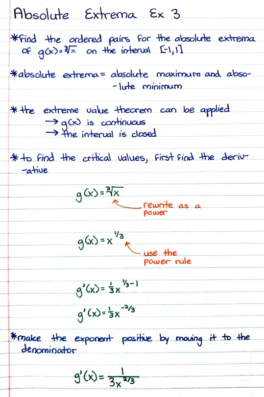

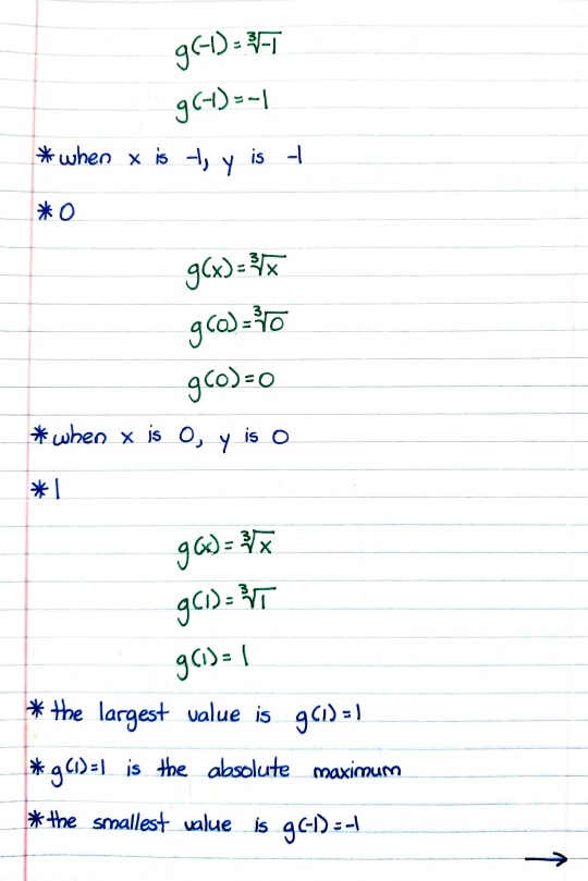
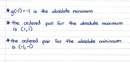
Patreon | Ko-fi
#studyblr#notes#math#maths#mathblr#math notes#maths notes#calculus#calculus notes#calculus ex#calculus example#absolute extrema#absolute extrema notes#absolute extrema ex#absolute extrema example#absolute minimum#absolute maximum
10 notes
·
View notes
Photo
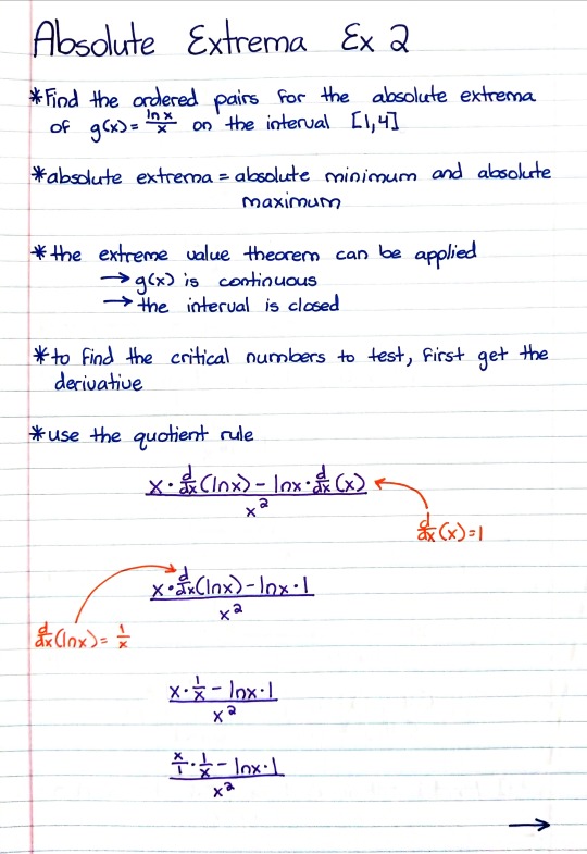
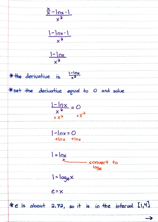

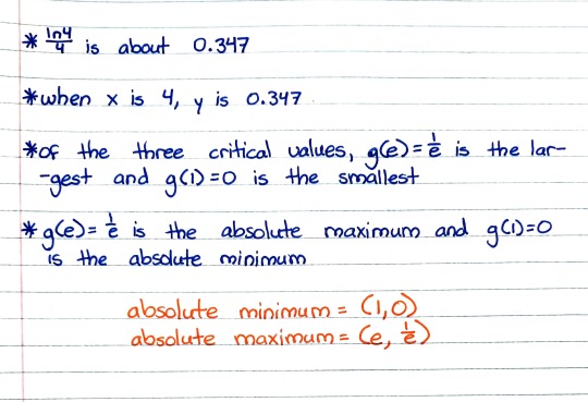
Patreon | Ko-fi
#studyblr#notes#math#maths#mathblr#math notes#maths notes#absolute extrema#absolute extrema example#absolute extrema ex#absolute extrema notes#calculus#calculus notes#calculus ex#calculus example#calculus i#calculus 1
10 notes
·
View notes
Photo

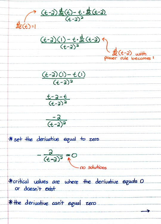


Patreon | Ko-fi
#studyblr#notes#math#maths#mathblr#maths notes#math notes#absolute extrema#absolute extrema notes#absolute extrema ex#absolute extrema example#calculus#calculus i#calculus 1#calculus 1 notes#calculus i notes#calculus ex#calculus example#calculus i ex#calculus i example
7 notes
·
View notes
Photo

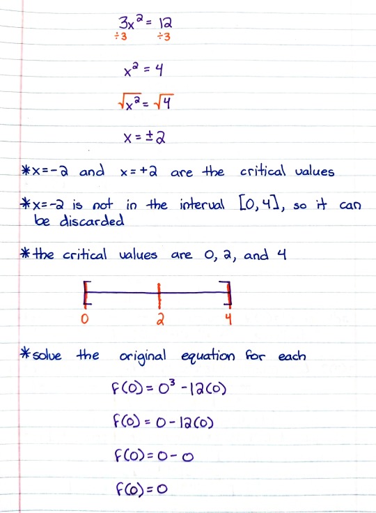
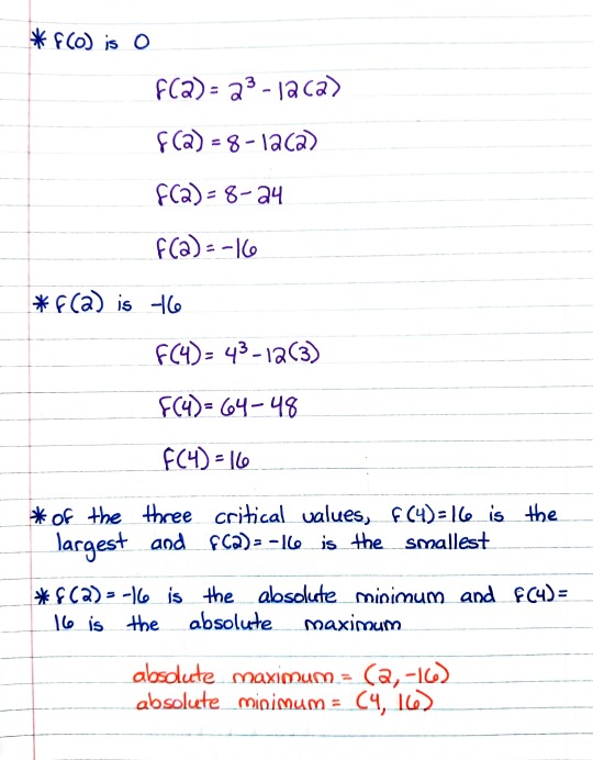
Patreon | Ko-fi
#studyblr#notes#math#maths#mathblr#math notes#maths notes#absolute extrema#absolute extrema notes#absolute extrema ex#absolute extrema example#calculus#calculus i#calculus 1#calculus ex#calculus example#calculus i example#calculus i ex#calculus 1 ex#calculus 1 example
6 notes
·
View notes
Photo

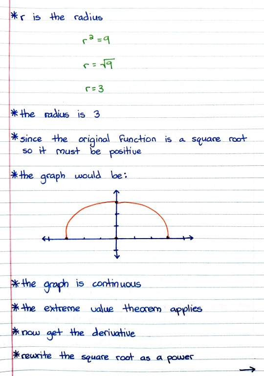


Patreon | Ko-fi
#math#studyblr#notes#maths#math notes#maths notes#calculus#calculus notes#calculus example#calculus ex#calculus 1#calc 1#calc#calc notes#calc example#calc ex#absolute extrema#extrema#graphs#graphing#graphing notes#calculus graphs#calculus 1 notes#calc 1 notes#absolute extrema ex#absolute extrema example
10 notes
·
View notes
Photo
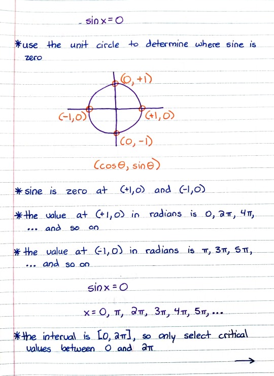
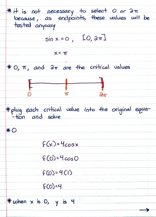
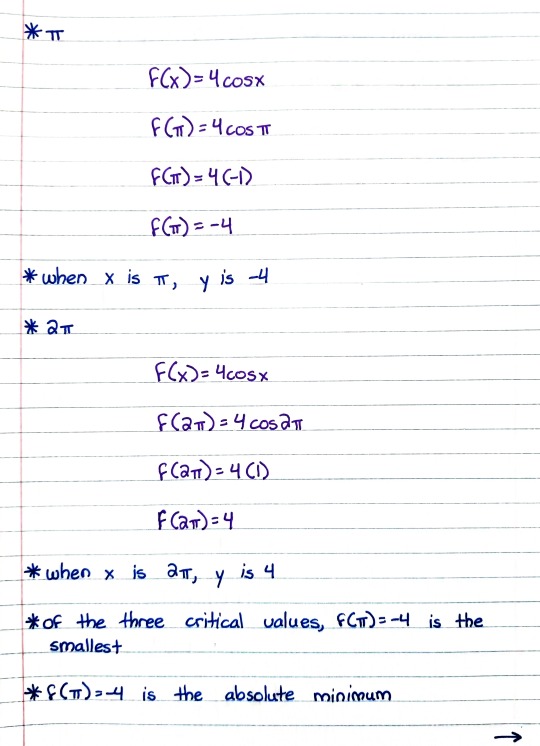
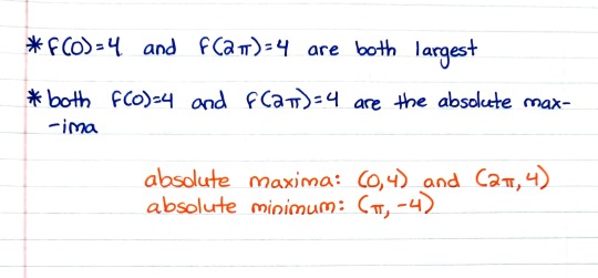
Patreon | Ko-fi
#studyblr#notes#math#maths#mathblr#math notes#maths notes#absolute extrema#trigonometry#trig#calculus#calculus notes#calculus example#calculus ex#calc#calc ex#calc example#calc notes#calculus i#calc i#calculus 1#calc 1#absolute maxima#absolute minima
6 notes
·
View notes
Photo
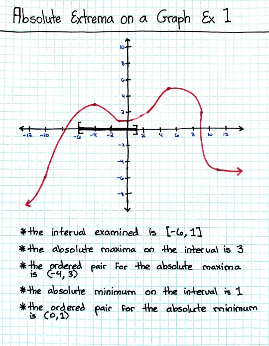
Patreon | Ko-fi
#studyblr#notes#math#maths#mathblr#math notes#maths notes#calculus#calculus i#calculus 1#calculus 1 notes#calculus i notes#calculus notes#calculus ex#calculus example#graphs#graphing#absolute extrema#absolute extrema notes#absolute extrema ex#absolute extrema example
2 notes
·
View notes
Last Seen Blogs

luxxurytaxxbeauty
Luxxury Taxx Beauty

taypinks
argumentative, antithetical dream girl

stockloanservice
Dover Management Services, Ltd

random0gener8r
Random Nought Generator

pembuatankalendermurahjakarta
Percetakan Kalender Jakarta